This exercise is an extension of Example 16.12 using the larger data set nels with 6,649 observations.

Question:

This exercise is an extension of Example 16.12 using the larger data set nels with 6,649 observations. Two estimated multinomial logit models are reported in Table 16.11. In addition to the variable GRADES, we have FAMINC = family income ( $\$ 1000$ units) and indicator variables for sex and race. The baseline group is students who chose not to attend college.

image text in transcribed

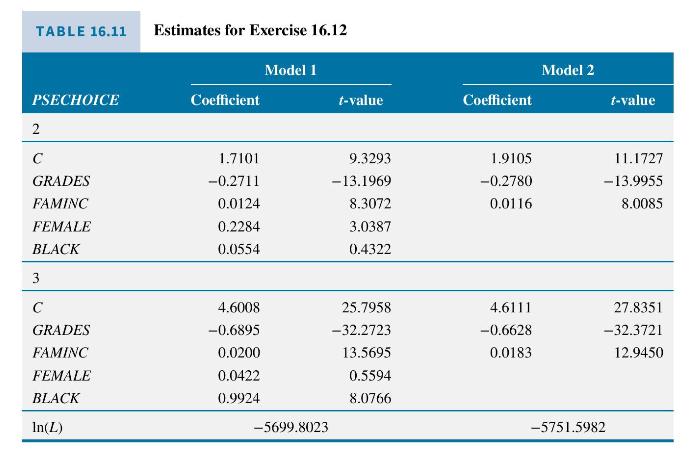
a. Which estimated coefficients are significant in Model 1? Based on the $t$-values, should we consider dropping FEMALE and BLACK from the model?

b. Compare the results of Model 1 to Model 2 using a likelihood ratio test. Using the $\alpha=0.01$ level of significance, can we reject the null hypothesis that the Model 1 coefficients of FEMALE and BLACK are zero?

c. Compute the estimated probability that a white male student with GRADES $=5$ (B) and FAMINC of $\$ 100,000$ will attend a 4-year college.

d. Compute the odds, or probability ratio, that a white male student with GRADES $=5(\mathrm{~B})$ and FAMINC of $\$ 100,000$ will attend a 4 -year college rather than not attend any college.

e. Compute the change in probability of attending a 4-year college for a white male student with median FAMINC $=\$ 100,000$ whose GRADES change from $5(\mathrm{~B})$ to $2(\mathrm{~A})$.

Data From Example 16.12:-

The National Education Longitudinal Study of 1988 (NELS:88) was the first nationally representative longitudinal study of eighth-grade students in public and private schools in the United States. It was sponsored by the National Center for Education Statistics. In 1988, some 25,000 eighth-graders and their parents, teachers, and principals were surveyed. In 1990, these same students (who were then mostly 10th graders, and some dropouts) and their teachers and principals were surveyed again. In 1992, the second follow-up survey was conducted of students, mostly in the 12th grade, but dropouts, parents, teachers, school administrators, and high school transcripts were also surveyed. The third follow-up was in 1994, after most students had graduated.

We have taken a subset of the total data, namely those who stayed in the panel of data through the third follow-up. On this group, we have complete data on the individuals and their households, high-school grades, and test scores, as well as their postsecondary education choices. In the data file nels_small, we have 1000 observations on students who chose, upon graduating from high school, either no college $(P S E C H O I C E=1)$, a 2 -year college $(P S E C H O I C E=2)$, or a 4-year college $(P S E C H O I C E=3)$. For illustration purposes, we focus on the explanatory variable GRADES, which is an index ranging from 1.0 (highest level, A+ grade) to 13.0 (lowest level, F grade) and represents combined performance in English, maths, and social studies.
Of the 1000 students, $22.2 \%$ selected not to attend a college upon graduation, $25.1 \%$ selected to attend a 2 -year college, and $52.7 \%$ attended a 4 -year college. The average value of GRADES is 6.53, with highest grade 1.74 and lowest grade 12.33. The estimated values of the parameters and their standard errors are given in Table 16.2. We selected the group who did not attend a college to be our base group, so that the parameters $\beta_{11}=\beta_{21}=0$.
Based on these estimates, what can we say? Recall that a larger numerical value of GRADES represents a poorer academic performance. The parameter estimates for

image text in transcribed

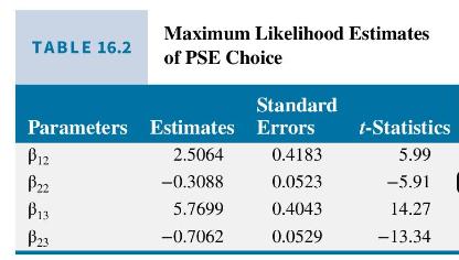
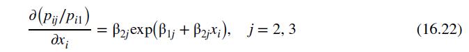
the coefficients of GRADES are negative and statistically significant. Using expression (16.22) on the effect of a change in an explanatory variable on the probability ratio, this means that if the value of GRADES increases, the probability that high-school graduates will choose a 2 -year or a 4-year college goes down, relative to the probability of not attending college. This is the anticipated effect, as we expect that a poorer academic performance will increase the odds of not attending college.
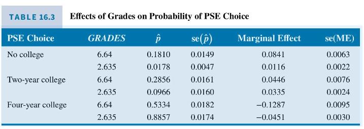
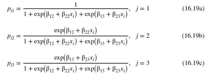
We can also compute the estimated probability of each type of college choice using (16.19) for given values of GRADES. In our sample, the median value of GRADES is 6.64, and the top 5th percentile value is $2.635 .{ }^{19}$ What are the choice probabilities of students with these grades? In Table 16.3, we show that the probability of choosing no college is 0.1810 for the student with median grades, but this probability is reduced to 0.0178 for students with top grades. Similarly, the probability of choosing a 2-year school is 0.2856 for the average student but is 0.0966 for the better student. Finally, the average student has a 0.5334 chance of selecting a 4-year college, but the better student has a 0.8857 chance of selecting a 4-year college.
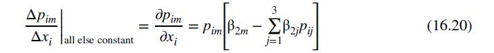
The marginal effect of a change in GRADES on the choice probabilities can be calculated using (16.20). The marginal effect again depends on particular values for GRADES, and we report these in Table 16.3 for the median and 5th percentile students. An increase in GRADES of one point (worse performance) increases the probabilities of choosing either no college or a 2-year college and reduces the probability of attending a 4-year college. The probability of attending a 4-year college declines more for the average student than for the top student, given the one-point increase in GRADES. Note that for each value of GRADES the sum of the predicted probabilities is one, and the sum of the marginal effects is zero, except for rounding error. This is a feature of the multinomial logit specification.

Data From Equation 16.19, 16.20 and 16.22:-