This exercise is an extension of Example 16.13. It is a conditional logit model of choice among 3 brands of soda: Coke, Pepsi, and 7-Up. The data are in the data file cola. As in the example, we choose Coke to be the base alternative, setting its alternative specific constant (intercept) to zero. We add to the model indicator variables FEATURE, indicating whether the product was "featured" at the time, and DISPLAY for whether there was a store display at the time of purchase. The model estimates are in Table 16.12.

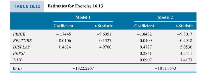
a. Using Model 1, calculate the probability ratio, or odds, of choosing Coke relative to Pepsi if Coke costs \(\$ 1.25\), Pepsi costs \(\$ 1.25\), Coke has a display but Pepsi does not, and neither are featured. Note that the model contains no alternative specific constants.

b. Using Model 1, calculate the probability ratio, or odds, of choosing Coke relative to Pepsi if Coke costs \(\$ 1.25\), Pepsi costs \(\$ 1.00\), Coke has a display but Pepsi does not, and neither are featured.

c. Compute the change in the probability of purchase of each type of soda if the price of Coke changes from \(\$ 1.25\) to \(\$ 1.50\), with the prices of Pepsi and 7-Up remaining at \(\$ 1.25\). Assume that a display is present for Coke, but not for the others, and none of the items is featured.

d. In Model 2, we add the alternative specific "intercept" terms for Pepsi and 7-Up to the Model 1. Calculate the probability ratio, or odds, of choosing Coke relative to Pepsi if Coke costs \(\$ 1.25\), Pepsi costs \(\$ 1.25\), Coke has a display but Pepsi does not, and neither are featured.

e. Using Model 2, compute the change in the probability of purchase of each type of soda if the price of Coke changes from \(\$ 1.25\) to \(\$ 1.50\), with the prices of Pepsi and 7 -Up remaining at \(\$ 1.25\). Assume that a display is present for Coke, but not for the others, and none of the items is featured.

f. The value of the log-likelihood function for the model in Example 16.13 is -1824.5621 . Test the null hypothesis that the coefficients of the marketing variables, FEATURE and DISPLAY, are zero, against the alternative that they are not, using a likelihood ratio test with \(\alpha=0.01\).

Data From Example 16.13:-

We observe 1822 purchases, covering 104 weeks and 5 stores, in which a consumer purchased 2-liter bottles of either Pepsi (34.6\%), 7-Up (37.4\%), or Coke Classic (28\%). These data are in the file cola. In the sample, the average price of Pepsi was \(\$ 1.23,7-\mathrm{Up} \$ 1.12\), and Coke \(\$ 1.21\). We estimate the conditional logit model shown in (16.22), and the estimates are shown in Table 16.4a.

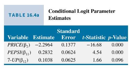
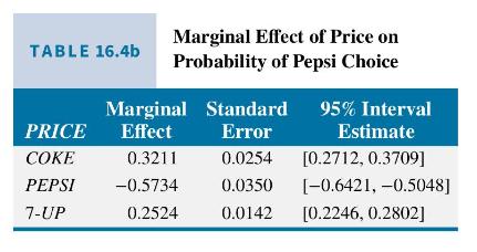
We see that all the parameter estimates are significantly different from zero at a \(10 \%\) level of significance, and the sign of the coefficient of PRICE is negative. This means that a rise in the price of an individual brand will reduce the probability of its purchase, and the rise in the price of a competitive brand will increase the probability of its purchase. Table \(16.4 \mathrm{~b}\) contains the marginal effects of price changes on the probability of choosing Pepsi. The marginal effects are calculated using (16.24) and (16.25) with prices of Pepsi, 7 -Up, and Coke set to \(\$ 1.00, \$ 1.25\), and \(\$ 1.10\), respectively. The standard errors are calculated using the delta method. Note two things about these estimates. First, they have the signs we anticipate. An increase in the price of Pepsi is estimated to have a negative effect on the probability of Pepsi purchase, while an increase in the price of either Coke or 7-Up increases the probability that Pepsi will be selected. Second, these values are very large for changes in probabilities because a "one-unit change" is \(\$ 1\), which then represents almost a \(100 \%\) change in price. For a 10 -cent increase in the prices the marginal effects, standard errors and interval estimate bounds should be multiplied by 0.10 .

As an alternative to computing marginal effects, we can compute specific probabilities at given values of the explanatory variables. For example, at the prices used for Table 16.4b, the estimated probability of selecting Pepsi is then

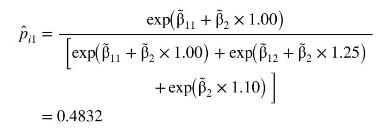
The standard error for this predicted probability is 0.0154 , which is computed via the delta method. If we raise the price of Pepsi to \(\$ 1.10\), we estimate that the probability of its purchase falls to 0.4263 ( \(\mathrm{se}=0.0135)\). If the price of Pepsi stays at \(\$ 1.00\) but we increase the price of Coke by 15 cents, then we estimate that the probability of a consumer selecting Pepsi rises by \(0.0445(\mathrm{se}=0.0033)\). These numbers indicate to us the responsiveness of brand choice to changes in prices, much like elasticities.

Transcribed Image Text:

TABLE 16.12 Estimates for Exercise 16.13 Model 1 Model 2 Coefficient t-Statistic Coefficient t-Statistic PRICE -1.7445 -9.6951 -1.8492 -9.8017 FEATURE -0.0106 -0.1327 -0.0409 -0.4918 DISPLAY 0.4624 4.9700 0.4727 5.0530 PEPSI 0.2841 4.5411 7-UP In(L) 0.0907 1.4173 -1822.2267 -1811.3543