We have (N=396) observations on employment at fast-food restaurants in two neighboring states, New Jersey and Pennsylvania.

Question:

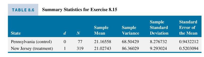
We have \(N=396\) observations on employment at fast-food restaurants in two neighboring states, New Jersey and Pennsylvania. In Pennsylvania, the control group \(d_{i}=0\), there is no minimum wage law. In New Jersey, the treatment group \(d_{i}=1\), there is a minimum wage law. Let the observed outcome variable be full-time employment \(F T E_{i}\) at comparable fast-food restaurants. Some sample summary statistics for \(F T E_{i}\) in the two states are in Table 8.6. For Pennsylvania, the sample size is \(N_{0}=77\), the sample mean is \(\overline{F T E}_{0}=\sum_{i=1, d_{i}=0}^{N_{0}} F T E_{i} / N_{0}\), the sample variance is \(s_{0}^{2}=\sum_{i=1, d_{i}=0}^{N_{0}}\left(F T E_{i}-\overline{F T E}_{0}\right)^{2} /\left(N_{0}-1\right)=\) \(S S T_{0} /\left(N_{0}-1\right)\), the sample standard deviation is \(\mathrm{s}_{0}=\sqrt{s_{0}^{2}}\), and the standard error of mean is \(\mathrm{se}_{0}=\sqrt{s_{0}^{2} / N_{0}}=s_{0} / \sqrt{N_{0}}\). For New Jersey, the definitions are comparable with subscripts " 1 ".

image text in transcribed

a. Consider the regression model \(F T E_{i}=\beta_{1}+\beta_{2} d_{i}+e_{i}\). The OLS estimates are given below, along with the usual standard errors (se), the White heteroskedasticity robust standard errors (robse), and an alternative robust standard error (rob2).

image text in transcribed

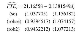
Show the relationship between the least squares estimates of the coefficients, the estimated slope and intercept, and the summary statistics in Table 8.6.

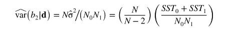
b. Calculate \(\widehat{\operatorname{var}}\left(b_{2} \mid \mathbf{d}\right)=N \hat{\sigma}^{2} /\left(N_{0} N_{1}\right)=\left(\frac{N}{N-2}\right)\left(\frac{S S T_{0}+S S T_{1}}{N_{0} N_{1}}\right)\), derived in Exercise 8.7(b). Compare the standard error of the slope using this expression to the regression output in part (a).

c. Suppose that the treatment and control groups have not only potentially different means but potentially different variances, so that \(\operatorname{var}\left(e_{i} \mid d_{i}=1\right)=\sigma_{1}^{2}\) and \(\operatorname{var}\left(e_{i} \mid d_{i}=0\right)=\sigma_{0}^{2}\). Carry out the Goldfeld-Quandt test of the null hypothesis \(\sigma_{0}^{2}=\sigma_{1}^{2}\) at the \(1 \%\) level of significance. [Hint: See Appendix C.7.3.]

d. In Exercise 8.7(e), we showed that the heteroskedasticity robust variance for the slope estimator is \(\widehat{\operatorname{var}}\left(b_{2} \mid \mathbf{d}\right)=\frac{N}{N-2}\left(\frac{S S T_{0}}{N_{0}^{2}}+\frac{S S T_{1}}{N_{1}^{2}}\right)\). Use the summary statistic data to calculate this quantity. Compare the heteroskedasticity robust standard error of the slope using this expression to those from the regression output. In Appendix 8D, we discuss several heteroskedasticity robust variance estimators. This one is most common and usually referred to as "HCE1," where HCE stands for "heteroskedasticity consistent estimator."

e. Show that the alternative robust standard error, rob2, can be computed from \(\widehat{\operatorname{var}}\left(b_{2} \mid \mathbf{d}\right)=\) \(\frac{S S T_{0}}{N_{0}\left(N_{0}-1\right)}+\frac{S S T_{1}}{N_{1}\left(N_{1}-1\right)}\). In Appendix 8D, this estimator is called "HCE2." Note that it can be written \(\widehat{\operatorname{var}}\left(b_{2} \mid \mathbf{d}\right)=\left(\hat{\sigma}_{0}^{2} / N_{0}\right)+\left(\hat{\sigma}_{1}^{2} / N_{1}\right)\), where \(\hat{\sigma}_{0}^{2}=\operatorname{SST}_{0} /\left(N_{0}-1\right)\) and \(\hat{\sigma}_{1}^{2}=\operatorname{SST}_{1} /\left(N_{1}-1\right)\). These estimators are unbiased and are discussed in Appendix C.4.1. Is the variance estimator unbiased if \(\sigma_{0}^{2}=\sigma_{1}^{2}\) ?

f. The estimator HCE1 is \(\widehat{\operatorname{var}}\left(b_{2} \mid \mathbf{d}\right)=\frac{N}{N-2}\left(\frac{S S T_{0}}{N_{0}^{2}}+\frac{S S T_{1}}{N_{1}^{2}}\right)\). Show that dropping the degrees of freedom correction \(N /(N-2)\) it becomes HCE0, \(\widehat{\operatorname{var}}\left(b_{2} \mid \mathbf{d}\right)=\left(\tilde{\sigma}_{0}^{2} / N_{0}\right)+\left(\tilde{\sigma}_{1}^{2} / N_{1}\right)\), where \(\tilde{\sigma}_{0}^{2}=S S T_{0} / N_{0}\) and \(\tilde{\sigma}_{1}^{2}=S S T_{1} / N_{1}\) are biased but consistent estimators of the variances. See Appendix C.4.2. Calculate the standard error for \(b_{2}\) using this alternative.

g. A third variant of a robust variance estimator, HCE3, is \(\widehat{\operatorname{var}}\left(b_{2} \mid \mathbf{d}\right)=\left(\frac{\hat{\sigma}_{0}^{2}}{N_{0}-1}\right)+\left(\frac{\hat{\sigma}_{1}^{2}}{N_{1}-1}\right)\), where \(\hat{\sigma}_{0}^{2}=\operatorname{SST}_{0} /\left(N_{0}-1\right)\) and \(\hat{\sigma}_{1}^{2}=S S T_{1} /\left(N_{1}-1\right)\). Calculate the robust standard error using HCE3 for this example. In this application, comparing HCE0 to HCE2 to HCE3, which is largest? Which is smallest?

Data From Exercise 8.7:-

Consider the simple treatment effect model \(y_{i}=\beta_{1}+\beta_{2} d_{i}+e_{i}\). Suppose that \(d_{i}=1\) or \(d_{i}=0\) indicating that a treatment is given to randomly selected individuals or not. The dependent variable \(y_{i}\) is the outcome variable. See the discussion of the difference estimator in Section 7.5.1. Suppose that \(N_{1}\) individuals are given the treatment and \(N_{0}\) individual are in the control group, who are not given the treatment. Let \(N=N_{0}+N_{1}\) be the total number of observations.

a. Show that if \(\operatorname{var}\left(e_{i} \mid \mathbf{d}\right)=\sigma^{2}\) then the variance of the OLS estimator \(b_{2}\) of \(\beta_{2}\) is \(\operatorname{var}\left(b_{2} \mid \mathbf{d}\right)=N \sigma^{2} /\left(N_{0} N_{1}\right)\). [Hint: See Appendix 7B.]

b. Let \(\bar{y}_{0}=\sum_{i=1}^{N_{0}} y_{i} / N_{0}\) be the sample mean of the outcomes for the \(N_{0}\) observations on the control group. Let \(S S T_{0}=\sum_{i=1}^{N_{0}}\left(y_{i}-\bar{y}_{0}\right)^{2}\) be the sum of squares about the sample mean of the control group, where \(d_{i}=0\). Similarly, let \(\bar{y}_{1}=\sum_{i=1}^{N_{1}} y_{i} / N_{1}\) be the sample mean of the outcomes for the \(N_{1}\) observations on the treated group, where \(d_{i}=1\). Let \(S S T_{1}=\sum_{i=1}^{N_{1}}\left(y_{i}-\bar{y}_{1}\right)^{2}\) be the sum of squares about the sample mean of the treatment group. Show that \(\hat{\sigma}^{2}=\sum_{i=1}^{N} \hat{e}_{i}^{2} /(N-2)=\left(S S T_{0}+S S T_{1}\right) /(N-2)\) and therefore that

image text in transcribed

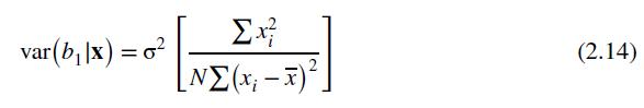
c. Using equation (2.14) find \(\operatorname{var}\left(b_{1} \mid \mathbf{d}\right)\), where \(b_{1}\) is the OLS estimator of the intercept parameter \(\beta_{1}\). What is \(\widehat{\operatorname{var}}\left(b_{1} \mid \mathbf{d}\right)\) ?

d. Suppose that the treatment and control groups have not only potentially different means but potentially different variances, so that \(\operatorname{var}\left(e_{i} \mid d_{i}=1\right)=\sigma_{1}^{2}\) and \(\operatorname{var}\left(e_{i} \mid d_{i}=0\right)=\sigma_{0}^{2}\). Find \(\operatorname{var}\left(b_{2} \mid \mathbf{d}\right)\). What is the unbiased estimator for \(\operatorname{var}\left(b_{2} \mid \mathbf{d}\right)\) ?

e. Show that the White heteroskedasticity robust estimator in equation (8.9) reduces in this case to \(\widehat{\operatorname{var}}\left(b_{2} \mid \mathbf{d}\right)=\frac{N}{N-2}\left(\frac{S S T_{0}}{N_{0}^{2}}+\frac{S S T_{1}}{N_{1}^{2}}\right)\). Compare this estimator to the unbiased estimator in part (d).

f. What does the robust estimator become if we drop the degrees of freedom correction \(N /(N-2)\) in the estimator proposed in part (e)? Compare this estimator to the unbiased estimator in part (d).

Data From Equation 2.14:-