In Section 3.8 .4 we derived an expression for the Gaussian posterior for a linear model within the context of the Olympic \(100 \mathrm{~m}\) data. Substituting \(\boldsymbol{\mu}_{0}=\) \([0,0, \ldots, 0]^{\top}\), we saw the similarity between the posterior mean

\[\boldsymbol{\mu}_{\mathbf{w}}=\frac{1}{\sigma^{2}}\left(\frac{1}{\sigma^{2}} \mathbf{X}^{\top} \mathbf{X}+\boldsymbol{\Sigma}_{0}^{-1}\right)^{-1} \mathbf{X}^{\top} \mathbf{t}\]

and the regularised least squares solution

\[\widehat{\mathbf{w}}=\left(\mathbf{X}^{\top} \mathbf{X}+N \lambda \mathbf{I}\right)^{-1} \mathbf{X}^{\top} \mathbf{t}\]

For this particular example, find the prior covariance matrix \(\boldsymbol{\Sigma}_{0}\) that makes the two identical. In other words, find \(\boldsymbol{\Sigma}_{0}\) in terms of \(\lambda\).

Data from Section 3.8 .4

.............

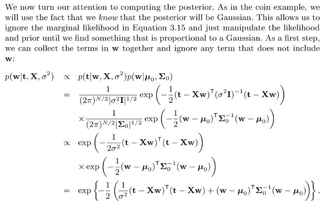
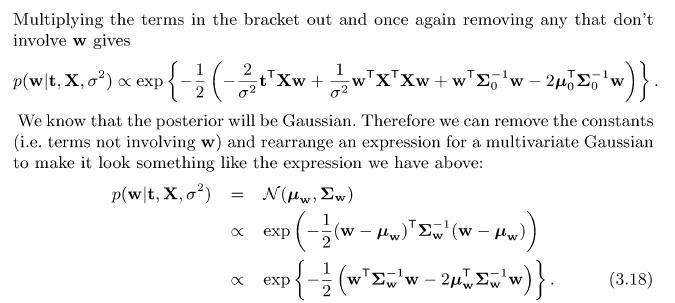
We now turn our attention to computing the posterior. As in the coin example, we will use the fact that we know that the posterior will be Gaussian. This allows us to ignore the marginal likelihood in Equation 3.15 and just manipulate the likelihood and prior until we find something that is proportional to a Gaussian. As a first step, we can collect the terms in w together and ignore any term that does not include W: p(wt, X,o) x p(t|w, X, o)p(wo, o) = 1 (2) N/2|21|1/2 1 (2)/2||1/2 1 x exp exp ((t xw) (o1)(t - Xw)) - ( (w - exp(-(-xw) (1-Xw)) (w-o)(w- - No)) (W - Ho)) ((w = exp - - 2 (t Xw)(t Xw) + (w )(w - 1 - Ho))}.