Use MATLAB to plot the variations of the damping constant \(c\) with respect to \(r, h\), and \(a\) as determined in Problem 1.72.

Data From Problem 1.72:-

In Problem 1.71, using the given data as reference, find the variation of the damping constant \(c\) when

a. \(r\) is varied from \(0.5 \mathrm{~cm}\) to \(1.0 \mathrm{~cm}\).

b. \(h\) is varied from \(0.05 \mathrm{~cm}\) to \(0.10 \mathrm{~cm}\).

c. \(a\) is varied from \(2 \mathrm{~cm}\) to \(4 \mathrm{~cm}\).

Data From Problem 1.71:-

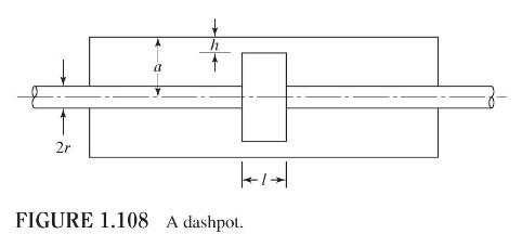
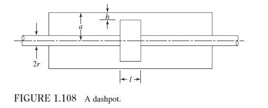
The damping constant \((c)\) of the dashpot shown in Fig. 1.108 is given by [1.27]:

\[c=\frac{6 \pi \mu l}{h^{3}}\left[\left(a-\frac{h}{2}\right)^{2}-r^{2}\right]\left[\frac{a^{2}-r^{2}}{a-\frac{h}{2}}-h\right]\]

Determine the damping constant of the dashpot for the following data: \(\mu=0.3445\) Pa-s, \(l=10 \mathrm{~cm}, h=0.1 \mathrm{~cm}, a=2 \mathrm{~cm}, r=0.5 \mathrm{~cm}\).

Transcribed Image Text:

2r FIGURE 1.108 A dashpot. Lat