We would like to solve the steady state heat transfer problem given by the drawing in Fig. 7.17. We have a composite solid material of area L_xL_y, with the left half having conductivity k₁ and the right half having conductivity k₂. The lower part of the material is in contact with a cold reservoir maintained at Tc, and the top half is maintained at two different hot temperatures, T_H,₁ and T_H,₂. The side walls of the material are insulating boundary conditions.

(a) Determine the set of dimensionless equations and boundary conditions needed to solve this problem. Your equations should involve a dimensionless temperature, θ = (T − T_C)/(T_H,1 − T_C) and length scales ˜x = x/L_x and ˜y = y/L_x. These naturally lead to a conductivity ratio k = k₁/k₂, a temperature ratio T_r = (T_H,₂ −T_C)/(T_H,₁ − T_C), and an aspect ratio L = L_y/L_x.

(b) We now want to write a MATLAB program to compute the temperature profile for given values of the parameters k, T_r, and L and the number of nodes nx used to discretize the geometry for one of the materials. Although there are many ways to construct the solution, use the grid in Fig. 7.18 (which is the easiest, if not the most efficient). The origin is in the upper left corner. The nodes for material 1 run from j = 1 to j = n_xn_y, where ny is the number of grid points needed for a given value of L with constant grid spacing Δx = Δy. The nodes for material 2 run from j = n_xn_y + 1 to j = 2n_xn_y. Note that both materials contain nodes at the interface, but they are at the same location. It is possible to reduce the number of nodes by substitution, but let’s use this slightly larger grid because it is conceptually simpler.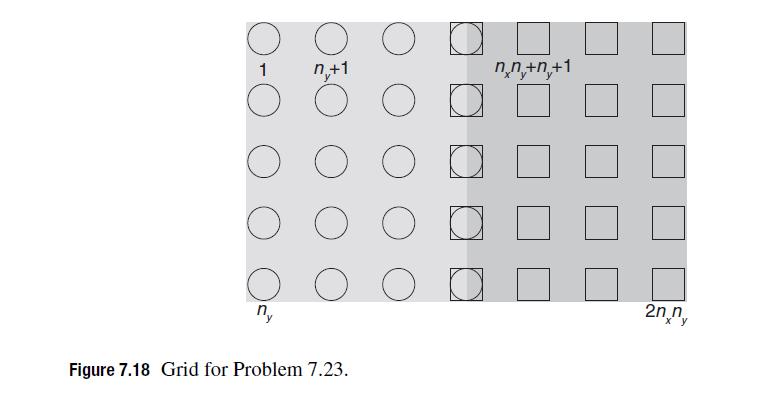

Convert the equations from part (a) into equations on this grid using finite difference. For the no-flux boundaries, use centered-finite differences. For the interface flux conditions, use forward or backward differences.

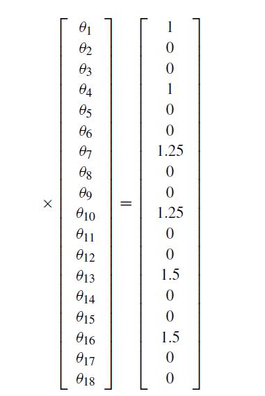
Write a MATLAB program that solves for the temperature profile leaving the values of k, T_r, L, and n_x as variables that you can easily change. To test your program, use k = 10, T_r = 1.5, and L = 0.5. Set n_x = 3, which is the smallest possible grid you can use. If you store the interface temperature conditions in the equations for the interface nodes in material 1 and the interface flux conditions in the equations for the interface nodes in material 2, you should have the following linear system to solve: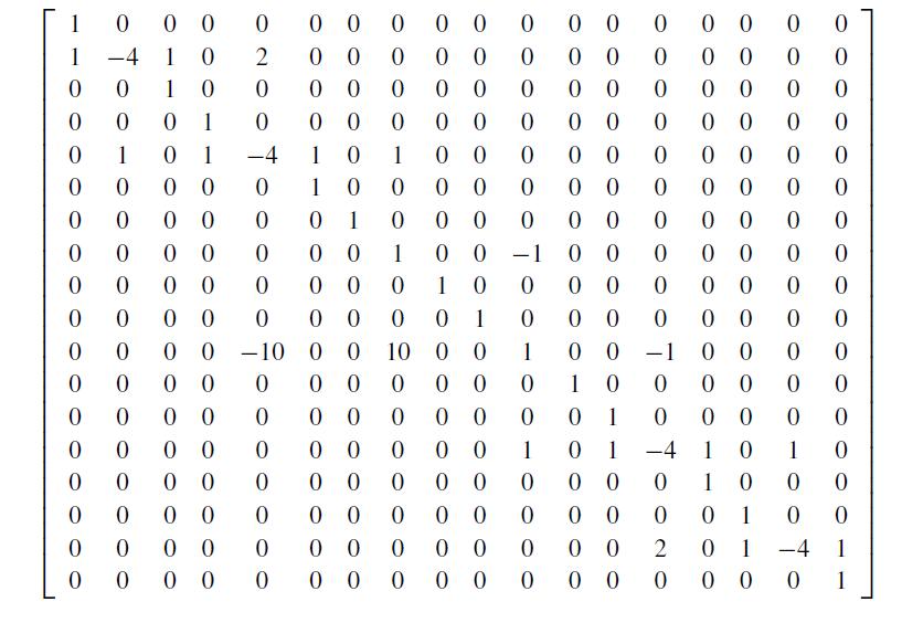

It is easiest to check your program using the Workspace environment in MATLAB, which will let you open up variables in a format similar to Excel. Once you know the program is working, use n_x = 32 to make a high-resolution plot of the temperature profile. You should use the surf function in MATLAB for the plot, and the view function to have it rotated to the proper orientation and elevation. Since it is a pain to add text to the plots, it is sufficient to get it into the same orientation as the figure in this assignment. Your program should automatically generate this figure.

(c) We now want to compare the numerical solution to the prediction of the resistor models. Recall that the resistor model would predict that the flux coming out of the bottom of each material would be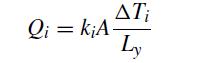

where A is the cross-sectional area. You can also compute the flux out of the bottom of material i = 1 and i = 2 by using backwards differences and then integrating across the boundary using Boole’s rule. (See Chapter 8.) Modify your program from part (b) to make this calculation for T_r values from 1.0 to 2.0 in increments of 0.1. Report your result as the ratio of Q from the numerical solution to the predicted value of Q for the resistor model for each of the materials. Your program should automatically generate the plot with axis labels, a legend, and a title. What does this plot tell you about the accuracy of the resistor model?

Transcribed Image Text:

1 O O ny о n+1 о о Figure 7.18 Grid for Problem 7.23. O O O о O A n¸n +n +1 2n_n xy