With the previous problem in mind, return to the autocorrelation of a sine function, shown in Fig. 11.51. Now suppose we have a signal composed of a great many sinusoidal components. Imagine that you take the autocorrelation of this complicated signal and plot the result (use three or four components to start with), as in part (e) of Fig. 11.51. What will the autocorrelation function look like when the number of waves is very large and the signal resembles random noise? What is the significance of the Ï„ = 0 value? How does this compare with the previous problem?

Fig. 11.51

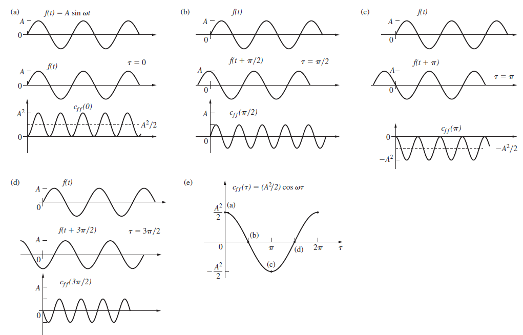
(a) (b) flt) (c) fit) f(t) = A sin wt A 0- A- fAt + 7/2) T = T/2 flt + T) flt) A - Cry(0) Crf(T/2) Cry(T) -A/2 (d) flt) (e) Crf(T) = (A/2) cos wT 42 |(a) fit + 37/2) %3D /2 (b) (d) (c) A Crp(37/2)