There is a great deal of disagreement concerning the shape of the AS curve. One view of the aggregate supply curve, the simple “Keynesian” view, holds that at any given moment, the economy has a clearly defined capacity, or maximum, output. This maximum output, denoted by Y_F, is defined by the existing labor force, the current capital stock, and the existing state of technology. If planned aggregate expenditure increases when the economy is producing below this maximum capacity, this view holds, inventories will be lower than planned, and firms will increase output, but the price level will not change. Firms are operating with underutilized plants (excess capacity), and there is cyclical unemployment.

Expansion does not exert any upward pressure on prices. However, if planned aggregate expenditure increases when the economy is producing near or at its maximum (Y_F), inventories will be lower than planned, but firms cannot increase their output. The result will be an increase in the price level, or inflation.

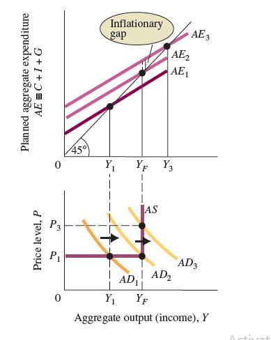
This view is illustrated in the figure. In the top half of the diagram, aggregate output (income) (Y) and planned aggregate expenditure (C + I + G ≡ AE) are initially in equilibrium at AE₁, Y₁, and price level P₁. Now suppose an increase in government spending increases planned aggregate expenditure. If such an increase shifts the AE curve from AE₁ to AE₂ and the corresponding aggregate demand curve from AD₁ to AD₂, the equilibrium level of output will rise from Y₁ to Y_F. (Remember, an expansionary policy shifts the AD curve to the right.) Because we were initially producing below capacity output (Y₁ is lower than Y_F), the price level will be unaffected, remaining at P₁.

Now consider what would happen if AE increased even further. Suppose planned aggregate expenditure shifted from AE₂ to AE₃, with a corresponding shift of AD₂ to AD₃. If the economy were producing below capacity output, the equilibrium level of output would rise to Y₃. However, the output of the economy cannot exceed the maximum output of YF.

As inventories fall below what was planned, firms encounter a fully employed labor market and fully utilized plants. Therefore, they cannot increase their output. The result is that the aggregate supply curve becomes vertical at Y_F, and the price level is driven up to P₃.

The difference between planned aggregate expenditure and aggregate output at full capacity is sometimes referred to  With planned aggregate expenditure of AE₁ and aggregate demand of AD₁, equilibrium output is Y₁. A shift of planned aggregate expenditure to AE₂, corresponding to a shift of the AD curve to AD₂, causes output to rise but the price level to remain at P₁. If planned aggregate expenditure and aggregate demand exceed Y_F, however, there is an inflationary gap and the price level rises to P₃. 

 As an inflationary gap. You can see the inflationary gap in the top half of the figure. At Y_F (capacity output), planned aggregate expenditure (shown by AE₃) is greater than Y_F. The price level rises to P₃ until the aggregate quantity supplied and the aggregate quantity demanded are equal.

Despite the fact that the kinked aggregate supply curve provides some insights, most economists find it unrealistic. It does not seem likely that the whole economy suddenly runs into a capacity “wall” at a specific level of output. As output expands, some firms and industries will hit capacity before others.

Questions

Why is the distance between AE₃ and AE₂ called an inflationary gap?

Transcribed Image Text:

Planned aggregate expenditure AE =C+I+G Price level, P P3 P₁ 45° Inflationary gap AE₂ AE1 Y₁ YF Y3 AS AD₂ AE 3 AD3 AD₁ Y₁ YF Aggregate output (income), Y Activat