1.8. Computer Challenge A problem of considerable contemporary importance is how to simulate a Brownian motion stochastic process. The invariance principal provides one possible approach. An infinite series expression that N. Wiener introduced may provide another approach. Let Z,,, Z,, ... be a series of independent standard normal random variables. The infinite series

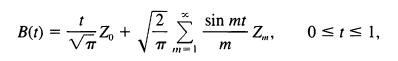
is a standard Brownian motion for 0 <_ t try to simulate a brownian motion stochastic process at least approximately by using finite of the form>

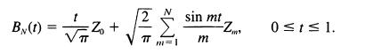
If B(t), 0

as an approximate standard Brownian motion. In what ways do these finite approximations behave like Brownian motion? Clearly, they are zero mean Gaussian processes. What is the covariance function, and how does it compare to that of Brownian motion? Do the gambler's ruin probabilities of (1.13) accurately describe their behavior? It is known that the squared variation of a Brownian motion stochastic process is not random, but constant:

This is a further consequence of the variance relation E[(OB)2] = At (see the remark in Section 1.2). To what degree do the finite approximations meet this criterion?

B(t) = + + 2 sin mt Z 0 1 1, m