Use the result in Problem 31.7 to determine the best fit parameters for the Vasicek model using
Question:
Use the result in Problem 31.7 to determine the best fit parameters for the Vasicek model using the same data as in Section 31.4 (see www-2.rotman.utoronto.ca/ hull/ VasicekCIR). Verify that the regression approach in Section 31.4 and the maximum-likelihood approach give the same answer.
Data From Problem 31.7:
Observations spaced at intervals \(\Delta t\) are taken on the short rate. The \(i\) th observation is \(r_{i}\) \((0 \leq i \leq m)\). Show that the maximum-likelihood estimates of \(a, b^{*}\), and \(\sigma\) in Vasicek's model are given by maximizing \[\sum_{i=1}^{m}\left(-\ln \left(\sigma^{2} \Delta t\right)-\frac{\left[r_{i}-r_{i-1}-a\left(b^{*}-r_{i-1}\right) \Delta t\right]^{2}}{\sigma^{2} \Delta t}\right)\]
Data From Section 31.4:
We will illustrate the estimation of parameters with Vasicek's model. The discrete version of the model in the real world is, from equation (31.13),
\[\Delta r=a\left(b^{*}-r\right) \Delta t+\sigma \epsilon \sqrt{\Delta t}\]
where \(\epsilon\) is a random sample from a standard normal distribution. Define \(r_{i}\) as the rate on day \(i\). Daily data on 3-month Treasury rates in the United States between January 4, 1982, and August 23, 2016, together with a worksheet for the analysis in this section, is on www-2.rotman.utoronto.ca/ hull/VasicekCIR. When we use this data to regress \(r_{i+1}-r_{i}\) against \(r_{i}\), we obtain
\[r_{i+1}-r_{i}=0.00000915-0.000545 r_{i}\]
with a standard error of 0.000754 .
We have about 250 observations per year, so that \(\Delta t=1 / 250\). Because \(0.00000915=\) \(0.00229 / 250,0.000545=0.136 / 250\), and \(0.000754=0.0119 / \sqrt{250}\), the regression result is equivalent to
\[\Delta r=(0.00229-0.136 r) \Delta t+0.0119 \epsilon \sqrt{\Delta t}\]
or
\[\Delta r=0.136(0.0168-r) \Delta t+0.0119 \epsilon \sqrt{\Delta t}\]
indicating that the best-fit parameters are \(a=0.136, b^{*}=0.0168\) (or \(1.68 \%\) ), and \(\sigma=0.0119\) (or \(1.19 \%\) ). Problem 31.15 shows that the same results are obtained using maximum-likelihood methods.
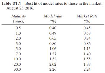
So far we have estimated the parameters for Vasicek's model in the real world. If the market price of risk is \(\lambda\), the previous section shows that in the risk-neutral world the parameters are \(a=0.136, b=0.168-0.0119 \lambda / a\), and \(\sigma=0.0119\). For a trial value of \(\lambda\), we can use equations (31.7), (31.8), and (31.10) to estimate zero-coupon rates as a function of maturity. Solver can then be used to determine the value of \(\lambda\) that minimizes the sum of squared errors between the zero-coupon rates given by the model and those in the market. This best-fit value of \(\lambda\) turns out to be \(-0.175 .{ }^{4}\) Table 31.1 compares the zero-coupon rates given by the model when this best-fit value of \(\lambda\) is used with those in the market.
The two-step estimation procedure we have used is a simple procedure and there has been no attempt to fit the term structure of interest rates at times other than today. In practice, researchers use more sophisticated econometric procedures. The parameters we have estimated for Vasicek's model are reasonable, but this will not always be the case. \({ }^{5}\)
The period of time over which parameters are estimated and the current shape of the term structure can have a big effect on the results obtained. Some judgment is necessary to determine the most appropriate data to use when a model such as Vasicek or CIR is estimated in practice.
Step by Step Answer: