1. The managing partner of an advertising agency believes that his company's sales are related to the industry sales. He uses Microsoft Excel's Data Analysis tool to analyze the last 4 years of quarterly data (i.e., = 60) with the following results: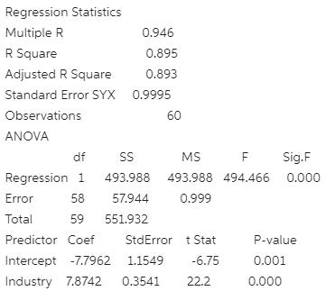  

a. What is the value of the quantity that the least squares regression line minimizes? Explain your answer.

b. What is the prediction of Y for a quarter in which X = 100? Show how you obtain your answer.

c. What is the value for the coefficient of determination?

d. What does the coefficient of determination tell you?

2. Your HR Director presents you the following data on your employees from a regression output

Dependent variable: Wage and Salary Income (INCWS)

Independent variable: a disability affecting work indicator

INCWS | Coefficient Std. Err. t P>|t| Beta

Work Disability | -9303.723 4475.500 -2.079 0.038 -0.070

constant | 37931.813 1416.073 26.787 0.000

a. Write the regression equation for the above output.

b. What information does the constant give you?

c. What information does the slope of the coefficient give you?
d. Write the null and alternative hypotheses to test whether or not disabled people earn less than non-disabled people.
e. At the 5% significance level, do disabled people earn less than non-disabled people?
f. At the 1% significance level, do disabled people earn less than non-disabled people?

3. Given below is the Excel output from regressing GPA on ACT scores using a data set of 75 randomly chosen students from a Big-Ten university, with GPA on a 5-point grading scale. 

   

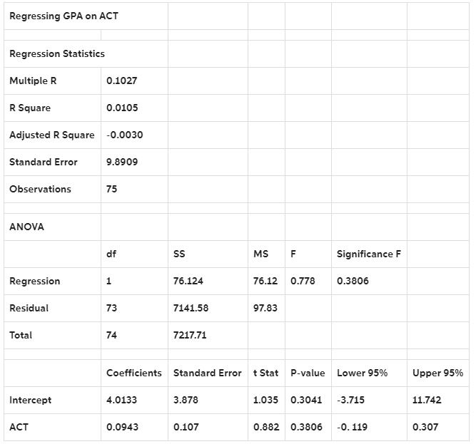
1. The interpretation of the coefficient of determination in this regression is 

A) 1.05% of the total variation of ACT scores can be explained by GPA.

B) ACT scores account for 1.05% of the total fluctuation in GPA.

C) GPA accounts for 1.05% of the variability of ACT scores.

D) None of the above.

4. Analysts at a major automobile company collected data on a variety of variables for a sample of 30 different cars and small trucks. Included among those data were the EPA highway mileage rating and the horsepower of each vehicle. The analysts were interested in the relationship between horsepower (x) and highway mileage (y). Given below is the Excel output from regressing starting miles per gallon (MPG) on number of horsepower for a sample of 30 students.

 Note: Some of the numbers in the output are purposely erased. 

  

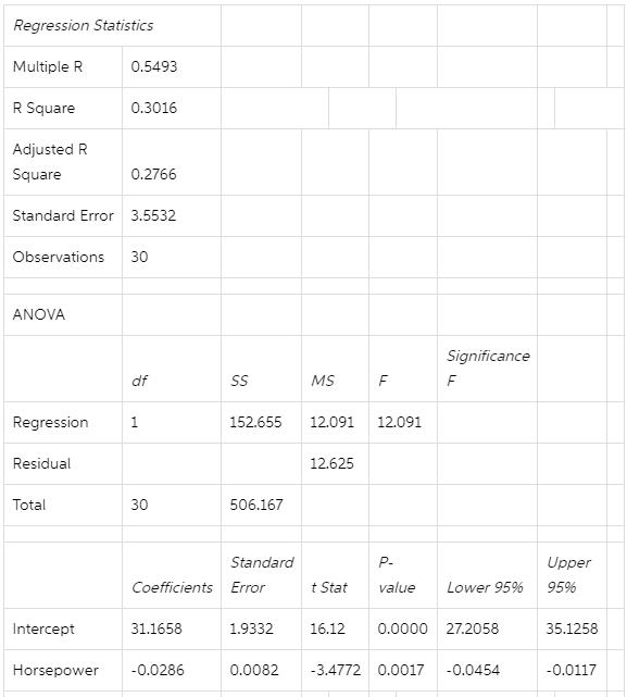
1. What is the estimated average change in MPG as a result of an extra unit of horsepower?  
2. What is the value of the measured t -test statistic and its p-value to test whether average MPG depends linearly on Horsepower?  

c) What is the error sum of squares (SSE) of the above regression? Show how you obtain your answer.

d) The 99% confidence interval for the average change in MPG as a result of increased horsepower is:

A) wider than [-0.0454, -0.0117].

B) narrower than [-0.0454, -0.0117].

C) wider than [27.2058, 35.1258].

D) narrower than [27.2058, 35.1258].

5. A shipping company believes that the variation in the cost of a customer’s shipment can be explained by differences in the weight of the package being shipped. To investigate whether this relationship is useful, a random sample of 20 customer shipments was selected, and the weight (in lb.) and the cost (in dollars, rounded) for each shipment were recorded. The following results were obtained:

1. Construct a scatter plot for these data. What, if any, relationship appears to exist between the two variables? 
2. Compute the linear regression model based on the sample data. Interpret the slope and regression coefficients.  

c) Test the significance of the overall regression model using a significance level of 0.05.

d) What percentage of the total variation in shipping cost can be explained by the regression model you developed in part b?

Weight (lbs.)	Cost (Dollars)
8	11
6	8
5	11
7	11
12	17
9	11
17	27
13	16
8	9
18	25
17	21
17	24
10	16
20	24
9	21
5	10
13	21
6	16
6	11
12	20

a) Construct a scatter plot for these data. What, if any, the relationship appears to exist between the two variables?
b) Compute the linear regression model based on the sample data. Interpret the slope and regression coefficients.
c) Test the significance of the overall regression model using a significance level of 0.05.
d) What percentage of the total variation in shipping cost can be explained by the regression model you developed in part b?

Regression Statistics Multiple R 0.946 R Square 0.895 Adjusted R Square 0.893 Standard Error SYX 0.9995 Observations 60 ANOVA df MS Sig.F Regression 1 493.988 493.988 494.466 0.000 Error 58 57.944 0.999 Total 59 551.932 Predictor Coef StdError t Stat P-value Intercept -7.7962 1.1549 -6.75 0.001 Industry 7.8742 0.3541 22.2 0.000