Question: 1 2 3 4 Simulation 5 6 7 8 9 10 11 12 13 6/14/22 20 21 22 23 24 25 26 Random Number

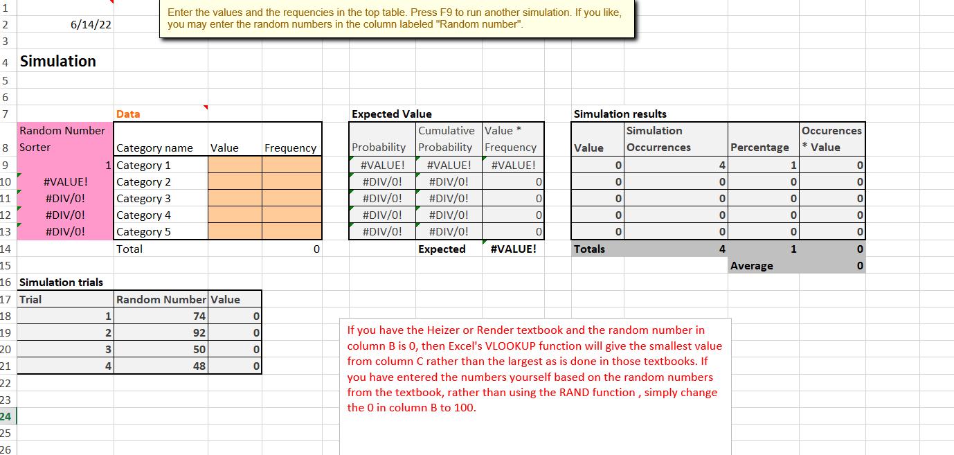
1 2 3 4 Simulation 5 6 7 8 9 10 11 12 13 6/14/22 20 21 22 23 24 25 26 Random Number Sorter #VALUE! #DIV/0!

1 2 3 4 Simulation 5 6 7 8 9 10 11 12 13 6/14/22 20 21 22 23 24 25 26 Random Number Sorter #VALUE! #DIV/0! #DIV/0! #DIV/0! 14 15 16 Simulation trials 17 Trial 18 19 Data 1 2 3 4 Enter the values and the requencies in the top table. Press F9 to run another simulation. If you like, you may enter the random numbers in the column labeled "Random number". Category name Value 1 Category 1 Category 2 Category 3 Category 4 Category 5 Total Random Number Value 74 92 50 48 0 0 0 0 Frequency 0 Expected Value Cumulative Value * Probability Probability Frequency #VALUE! #VALUE! #VALUE! #DIV/0! #DIV/0! #DIV/0! #DIV/0! #DIV/0! #DIV/0! #DIV/0! #DIV/0! Expected 0 0 0 0 #VALUE! Simulation results Simulation Occurrences Value Totals 0 0 0 0 0 4 0 0 0 0 4 If you have the Heizer or Render textbook and the random number in column B is 0, then Excel's VLOOKUP function will give the smallest value from column C rather than the largest as is done in those textbooks. If you have entered the numbers yourself based on the random numbers from the textbook, rather than using the RAND function, simply change the 0 in column B to 100. Percentage Average 1 0 0 0 0 1 Occurences * Value 0 0 0 0 0 0 0

Step by Step Solution

★★★★★

3.46 Rating (166 Votes )

There are 3 Steps involved in it

1 Expert Approved Answer

Step: 1 Unlock

SOLUTION It looks like you have a table set up with the following columns 1 Category name 2 ... View full answer

Question Has Been Solved by an Expert!

Get step-by-step solutions from verified subject matter experts

Step: 2 Unlock

Step: 3 Unlock

Students Have Also Explored These Related Accounting Questions!

(i) 8 9 10 11 12 (ii) 7 9 10 11 13 (iii) 7 8 10 12 13 (a) Without doing any computations, order the data sets according to increasing value of standard deviations. (b) Why do you expect the...

Accounting March February 6 7 8 9 Master Schedule for Day-Glo Solar Panels January 1 2. 3 4 5 120 95 100 120 135 140 102 125 115 120 165Solar panel product structure tree 1 Solar Panel Week...

Evertight a leading manufacturer of quality nails produces 1 2 3 4 and 5 inch nails clavos for various uses In the production process if there is an overrun or the nails are slightly defective they...

Repeat Example 11.9, with the entire range of methanol feed-stage locations. Compare your results for isobutene conversion with the values shown infigure. 0.9 0.8 0.7 0.6 0.5 0.4 0.3 0.2 0.1E 1 2 3 4...

The accompanying graph (bottom of this page) summarizes the demand and costs for a firm that operates in a monopolistically competitive market.a. What is the firm??s optimal output?b. What is the...

If the region shown in the figure is rotated about the -axis to form a solid, use the Midpoint Rule with n = 5 to estimate the volume of the solid. 3. 1 2 3 4 5 6 7 8 9 10 11 12 2.

You are one of three carpenters assigned to complete a short construction project. Right before the start of the project, one of your fellow carpenters was hospitalized and will not be available to...

The Langborne Hotel is concerned about the number of people who book rooms by telephone but do not actually turn up. The following table shows the numbers of people who have done this over the past...

1. What is your opinion of the level at which the data are being collected? What are some of the advantages of collecting data at this level? 2. Aggregate the original data for October as you see...

Use the accompanying graph to answer the questions that follow. a. Suppose this monopolist is unregulated.(1) What price will the firm charge to maximize its profits?(2) What is the level of consumer...

Which fin is least likely to exhibit a 1 - D temperature profile?

The system below is in balance. In the CB string, the force modulus is 2400 N. The mass suspended from point D is 60 kg. The centre of mass of the rod shall be 2,0 m from point A. wwwwww B 0.5 m D 3...

Telehealth is increasingly being used by counselors. Counselors report they struggle with providing quality counseling to children through telehealth. Read "A Randomized Controlled Trial of...

Solville Motors Co. makes motorcycles Managment wants to estimate overhead costs to plan its operations. A recent trade publication revealed that overhead costs tend to vary with machine hours. to...

Employment Law Garcia v. Spun Steak Co., 998 F.2d 1480 (9th Cir. 1993) The defendant, Spun Steak Co., employs 33 workers, 24 of whom are Spanish-speaking. Two of the Spanish speakers speak no...

Solve the symbolic expression for the bending moment in case III. Also, solve the expression for the bending moment in case II in range of [0, L/2]. I II III 11111 x y L/2 * q 2q L/2 B *

intermediate accounting 1, chapter 3 Problem 3-1

If the jobs displayed in Table 18.24 are processed using the earliestdue-date rule, what would be the lateness of job C? TABLE 18.24 Processing Times and Due Dates for Five Jobs Job C D E...

After transforming each of the raw scores below into a z score, transform each z score into a standard score with a mean of 50 and a standard deviation of 10. Standard Raw Mean Deviation Exam Score...

Identifying the treatment group with 1 , specify both the null and alternative hypotheses for each of the following studies. Assume that the data from all these studies will be analyzed with...

Does the statement typify descriptive statistics (because it describes sets of actual observations) or inferential statistics (because it generalizes beyond collections of actual observations)? 1....

Marta borrowed $1750 from Jasper on November 15, 2008, and agreed to repay the debt with simple interest at the rate of 7.4% on June 3, 2009. How much interest was owed on June 3?

Paul has $20,000 to invest for six months. For this amount, his bank pays 3.3% on a 90-day GIC and 3.5% on a 180-day GIC. If the interest rate on a 90-day GIC is the same three months from now, how...

Sheldrick Contracting owes Western Equipment $60,000 payable on June 14. In late April, Sheldrick has surplus cash and wants to settle its debt to Western Equipment, if Western will agree to a fair...