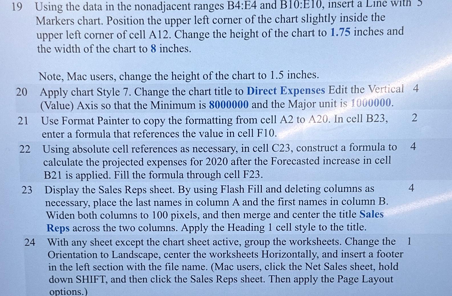
$19$ Using the data in the nonadjacent ranges B$4$:E$4$ and B$10$:E$10,$ insert a Line with $5$ Markers chart. Position the upper left corner of the chart slightly inside the upper left corner of cell A$12.$ Change the height of the chart to $1\mathrm{.}75$ inches and the width of the chart to $8$ inches.

Note, Mac users, change the height of the chart to $1\mathrm{.}5$ inches.

$20$ Apply chart Style $7.$ Change the chart title to Direct Expenses Edit the Vertical $4($Value$)$ Axis so that the Minimum is $8000000$ and the Major unit is $1000000.$

$21$ Use Format Painter to copy the formatting from cell A$2$ to A$20.$ In cell B$23,$

$2$

enter a formula that references the value in cell F$10.$

$22$ Using absolute cell references as necessary, in cell $C23,$ construct a formula to

$4$

calculate the projected expenses for $2020$ after the Forecasted increase in cell B$21$ is applied. Fill the formula through cell F$23.$

$23$ Display the Sales Reps sheet. By using Flash Fill and deleting columns as

$4$

necessary, place the last names in column A and the first names in column B$.$ Widen both columns to $100$ pixels, and then merge and center the title Sales Reps across the two columns. Apply the Heading $1$ cell style to the title.

$24$ With any sheet except the chart sheet active, group the worksheets. Change the $1$ Orientation to Landscape, center the worksheets Horizontally, and insert a footer in the left section with the file name. $($Mac users, click the Net Sales sheet, hold down SHIFT, and then click the Sales Reps sheet. Then apply the Page Layout options.$)$