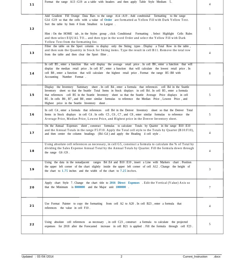
Question: 11 Format the range A13 :G19 as a table with headers and then apply Table Style Medium 5. Add Gradient Fill Orange Data Bars to

11 Format the range A13 :G19 as a table with headers and then apply Table Style Medium 5. Add Gradient Fill Orange Data Bars to the range A14 :A19 . Add conditional formatting to the range G14 :G19 so that the cells with a value of Order are formatted as Yellow Fill with Dark Yellow Text. Sort the table by Item # from Smallest to Largest 12 Hint : On the HOME tab , in the Styles group , click Conditional Formatting . Select Highlight Cells Rules and then select EQUAL TO... and then type in the word Order and select the Yellow Fill with Dark Yellow Text from the formatting list. Filter the table on the Sport column to display only the Skiing types . Display a Total Row in the table , and then sum the Quantity in Stock for Skiing items. Type the result in cell BI1. Remove the total row 13 from the table and then clear the Sport filter . In cell BS , enter a function that will display the average retail price . In cell Bo , enter a function that will display the median retail price . In cell B7 , enter a function that will calculate the lowest retail price . In 14 cell BB, enter a function that will calculate the highest retail price . Format the range B5 : BB with Accounting Number Format . Display the Inventory Summary sheet . In cell B4, enter a formula that references cell B4 in the Seattle Inventory sheet so that the Seattle Total Items in Stock displays in cell B4 . In cell BS, enter a formula 15 that references cell B5 in the Seattle Inventory sheet so that the Seattle Average Price displays in cell 5 B5 . In cells B6, B7 , and B8, enter similar formulas to reference the Median Price , Lowest Price , and Highest price in the Seattle Inventory sheet . In cell C4, enter a formula that references cell B4 in the Denver Inventory sheet so that the Denver Total 16 Items in Stock displays in cell C4. In cells C5, C6, C7, and CB, enter similar formulas to reference the Average Price, Median Price, Lowest Price, and Highest price in the Denver Inventory sheet. On the Annual Expenses sheet , construct formulas to calculate Totals by Quarter in the range B10 :E10 and the Annual Totals in the range F5:F10. Apply the Total cell style to the Totals by Quarter (B10:F10), 17 and then center the column headings (B4 :G4 ) and apply the Heading 4 cell style . Using absolute cell references as necessary, in cell G5, construct a formula to calculate the % of Total by dividing the Sales Expense Annual Total by the Annual Totals by Quarter. Fill the formula down through the range G6:G9 Using the data in the nonadjacent ranges B4:E4 and B10 :E10 , insert a Line with Markers chart . Position the upper left corner of the chart slightly inside the upper left corner of cell A12 . Change the height of 19 the chart to 1.75 inches and the width of the chart to 7.25 inches. 3 Apply chart Style 7. Change the chart title to 2016 Direct Expenses . Edit the Vertical (Value) Axis so 20 that the Minimum is 8000000 and the Major unit 1000000 21 Use Format Painter to copy the formatting from cell A2 to A20 . In cell B23 , enter a formula that references the value in cell F10 . 2 2 Using absolute cell references as necessary , in cell C23 , construct a formula to calculate the projected 5 expenses for 2018 after the Forecasted increase in cell B21 is applied . Fill the formula through cell F23 . Updated : 03 /04 /2014 Current_Instruction .docx
Step by Step Solution
There are 3 Steps involved in it

Get step-by-step solutions from verified subject matter experts


