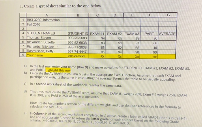
Question: 1. Create a spreadsheet similar to the one below. B D E F G 1 BISI 3230: Information 2 Fall 2016 3 4 STUDENT NAMES

1. Create a spreadsheet similar to the one below. B D E F G 1 BISI 3230: Information 2 Fall 2016 3 4 STUDENT NAMES 5 Thomas Steven 6 Alexander Suzette 7 Richards Billy Joe 8 Rasmussen Betty 9 Your name STUDENT ID EXAM #1 EXAM #2 EXAM #3 999-25-5683 94 65 89 999-52-6938 93 91 97 998-71-2838 55 62 65 997-74-4447 95 94 90 XOX-XX-XXXX Xx Xx PART AVERAGE 90 80 40 90 XX a) In the last row, enter your name (Row 9) and make up values for STUDENT ID, EXAM #1, EXAM #2, EXAM #3, and PART. Highlight this row. b) Calculate the AVERAGE in column G using the appropriate Excel Function. Assume that each EXAM and participation weights the same in calculating the average. Format the table to be visually appealing. c) In a second worksheet of the workbook, reenter the same data. d) This time, to calculate the AVERAGE score, assume that EXAM #1 weighs 20%, Exam # 2 weighs 25%, EXAM #43 is 30%, and PART is 25% of the average score. Hint: Create Assumptions section of the different weights and use absolute references in the formula to calculate the AVERAGE e) In Column Hof the second worksheet completed in c) above, create a label called GRADE (that is in Cell H4). Use and appropriate function to return the letter grade for each student based on the following Grade criteria: > 90.00: A, 80-89.99: B, 70-70.99: C, 60-60.99: D, and

Step by Step Solution

There are 3 Steps involved in it

1 Expert Approved Answer

Step: 1 Unlock blur-text-image

Question Has Been Solved by an Expert!

Get step-by-step solutions from verified subject matter experts

Step: 2 Unlock

Step: 3 Unlock

Students Have Also Explored These Related General Management Questions!

Please sir do it perfectly EXCEL EXERCISE #1: Grade Sheet 1. Enter the information in the spreadsheet below. Be sure that the information is entered in the same cells as given, or the formulas below...

Please help with steps seventeen through 21. Hokie Fitness Equipment & Accessories, Inc. is a retailer that sells fitness equipment and accessories. The manager of Hokie Fitness Equipment &...

Please help with steps seven through sixteen. Hokie Fitness Equipment & Accessories, Inc. is a retailer that sells fitness equipment and accessories. The manager of Hokie Fitness Equipment &...

My company for this project is Amazon. I have 3 pages on the xcel file to fill out. Included are the instructions and the financial statements for the project. Due to a family tragedy I missed a...

Background: Your company has just acquired a new subsidiary that makes two products, Clodhopper and Clodbuster. The Clodhopper is intended for the general consumer market and its demand is higher and...

Management information system and analysis homework Please follow the instruction step by step Thank you so much for help AutoSave . Off ) H Database Basics - Chuckies Supplies Sales - Saved sayed...

Please help answer part a to f: Ensure the following Corrections are used: There is an error in Part B. should read the bottom right corner in cell D38. There is an error in Part D. should read 2017...

Hello. Can you help with this four question problem? Case PRIVATE EQUITY CASE: MERGER CONSOLIDATION The questions below COMBINE the Ohio & Maryland PT acquisitions as if they are a single c Learning...

I need, I am working on GENERAL ELECTRIC AND UNITED TECHNOLOGIES CORP, I need help GE and UTC Financial Statements Forecast for the next 5 year using the attachment. Throughout this course you will...

File Home Insert Draw Page Layout Formulas Data Review View Help Comments Share MS Sans Serif AutoSum 10 ~ A == ale Wrap Text General AT TT 28 X Cut LO Copy Format Painter Fill Paste BI U Insert...

Panther Company acquires an 80% interest in Sargo Company for $272,000 in cash on January 1, 2011, when Sargo Company has the following balance sheet: The excess of the price paid over book value is...

The research topic is IT metrics applying measurement to solving a business problem.

4 . y l n sonunda 2 0 0 0 $ ve 1 0 . y l n sonunda 5 0 0 0 $ l k getirisi olan bir yat r m i in yat r mc 3 . y l n sonunda bu yat r m n masraflar i in 3 0 0 0 $ ve art bir miktar daha ek deme yapmak...

As the manager of Smith Construction, you need to make a decision on the number of homes to build in a new residential area where you are the only builder. Unfortunately, you must build the homes...