1) explain this 3 figure?

2)HOW DO YOU DEFINE THE OPTIMAL CAPITAL STRUCTURE FOR THE PROJECT?

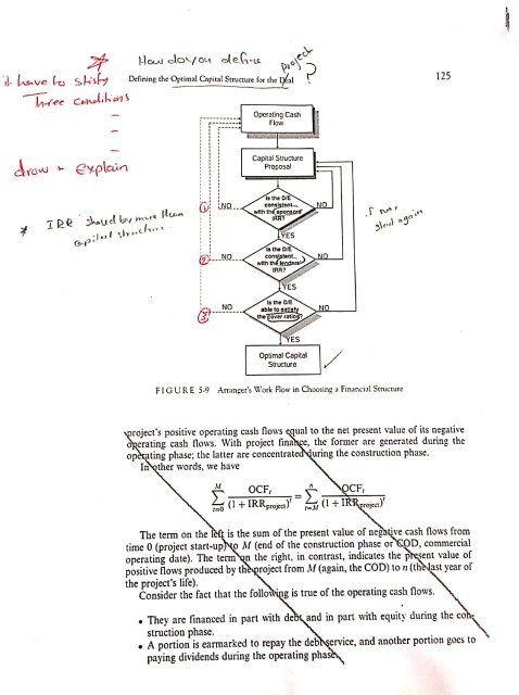
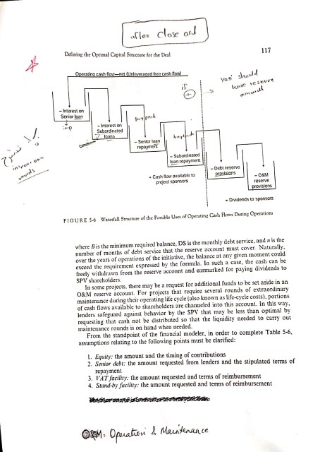
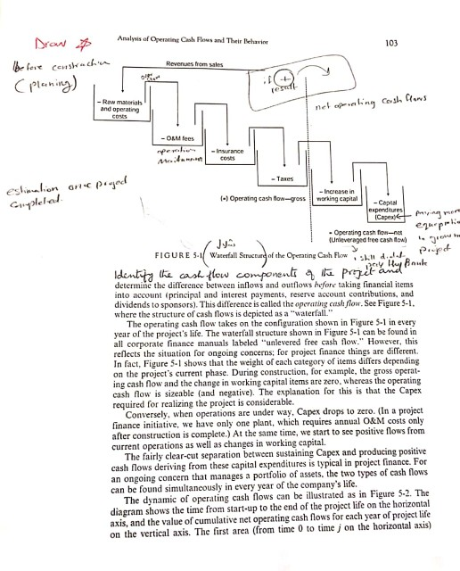
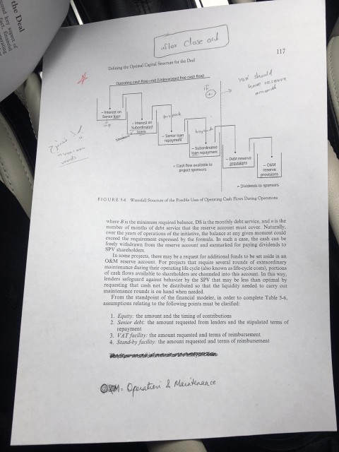
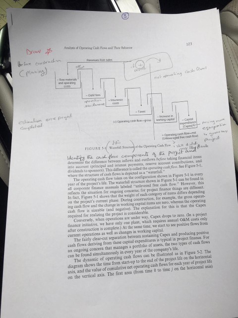
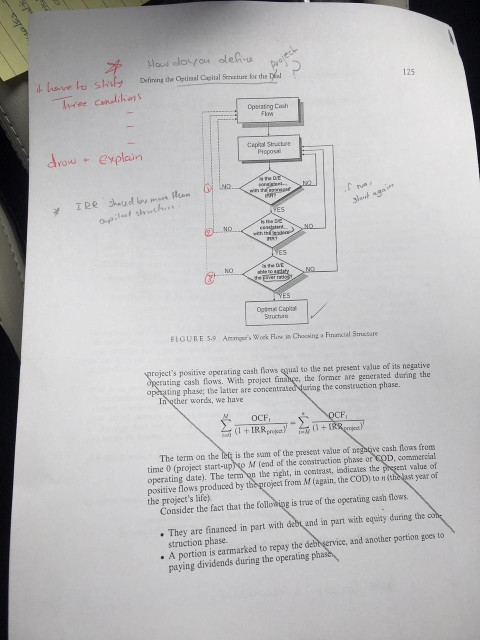
I fler close ad Defring the Opinal Coital Strecnze for the Deal ir htarest on repayme fow sealable to where 8 is the minimum requirod halance, DS is the monthly debt service, and n is the number of months of debl service that the reserve account must cover. Naturally over the years of operatioes of the initiative, the balance at any given moment could eeeed the requirement espeesod by the frmula. In such a case, the cash e be freely withdrawn trom the reserve account and carmarked for paying dividends to SPV shareholders La some pcojects, there may be a request for adsitional funds to be set aside ia an 0&M reserve account. For projects that require several rounds of extraordinary maintenance during their operating lite cycle (also known as tife-cycle coszs), portions of cash tlous available to sharebolders are channcled into this account, In this way, enders safeguard against behasior by the SPV that may be less than optimal by requesting that cash not be distributed so that the quidity needed to carry maintenance rounds is en hand when needed From the standpoint of the financial modeler, in order to oomplete Table 5-6 assumptions relating to the following points mest be clarificd Equiry: the amount and the timing of ocatributioas 2. Senlor deht the amount requested from lenders and the stipulased terms of repaymen 4Saby facity the amount requested and terms of reimbursement Pepun te ra Analysis of Operating Cesh Rows and Ther Fehaice 103 CPlahing) hoeise in Operating cush fow-ut FIGURE 3-1 Waterfall determin the difference between inlows acd outilows before taking financial ilems into account (principal and interest payments, reserve accoumt contributions, and dividends to sponsors). This differ ence is called the operating cash fiow, See Figure 5-1 where the structure of cash flows is depicted as a "waterfall The operating cash flow takes on the configuration shown in Figure 5-1 in every year of the project's life. The waterfall structure shown in Figure 5-1 can be Sound i all corporate finance manuals labeled unlevered free cash flow. Howeves, this reflects the situation for ongoing concens, for project finanoe things are differemt. ln fact, Figure 5-1 shows that ihe weight of each category of items differs depending on the project's current phase. During construction, for example, the gross operat- ing cash flow and the change in working capital items are zero, whereas the operating cash flow is sizcable land negative) The explanation for this is that the Capex required for realizing the project is considerable Conversely, when operations are under way, Capex drops to zero. (In a project finance initiative, we have only one plans, wlich reqaires annual O&M costs only after construction is complete.) At the same time, we start to see pesitive flows from current operatnsas wel as changes in wocking capital. The fairly clear-cut separation between sustaining Capex and producing paitive cash flows deriving from these capital expenditures is typical in project finance. For an ongoing concern that manages a poetfolio of assets, the two types of cash flows can be found simultaneously in every year of the company's ife. The dynamic of operating cash flows can be illustrated as in Figure 52. Tbe diagram shows the time from start-up to the end of the project life on the horizootal axis, and the value of cumulative set operating cash flows for each year of projoct life on the vertical axis. The fitst area (from time 0 to time j on the horizontal axis) Defining the Optinal Capital Strecture fot the T 125 Operztirg Canh apizal Strucure Pioposs explain Sructre FIGURE 5.9 AaersWork Fluw in Chooing s Finaclal Smature roject's positive operating cash flows qual to the net present value of its negative perating cash flows. With project timange, the former are genetated during the ophating phase; the latier are concentrated uring the construction phase. In qther words, we have OCF The term on the lot is the sum of the present value of negative cash florws from time 0 (project start-upto M (end of the construction phase or COD, commercial operating date). The term on the right, in contrast, ndicales the present value of positive flows produced by theproject from M lagain, the COD) to n thest year of the project's life) Consider the fact that the following is true of the operating cash flows struction phase. paying dividends during the operating phas .They are financed in part with deb and in part with equity during the . A portion is carmarked to repay the dehheervice, and another portion goes to Defining the Optimal Capital Structure for ehve Operating Cash Captal Suucure xplain FIGURE 5.9 Amanger's Work Flow in Choosing a Financial Seucture s positive operating cash nows equal to the net present value of its negative cash flows. With project phase te latter are the former are generated during the uring the construction phase. e cash flows from The term on the eis the sum of the present value of time 0 (project start-upo M (end of the construction phase or COD, commercial value of operating date). The term on the right, in contrast, indicates the positive from M (again, the COD) to n(t year of g is true of the operating cash flows. Consider the fact that the They are financed in part with debt and in part with equity during the c . A portion is earmarked to repay the de and another portion goes to paying dividends during the operating fler close od Defining the Opcimal Capital Suructere for the Deal ir Serior lar Serigr loan Subord nated Cash ow aalbe preject sponsors reseve Dridenes to spamiors FIGURE $-6 Watetfall Struure of theonile U oOtating Ca Flnes During Operatices where B is the minimum required balance, DS is the monthly debt service, and m is the number of months of debi service that the reserve account must cover Naturaly over the years of operations of the initiatve, the balance at any given moment could esceed the requirement expressed by the formula. In such a case, the cash can be freely withurawn from the reserve account and earmarked for paying divideads to SPV shareholders In some projects, there may be a request for additional funds to be set aside in an O&M reserve account. For equire several rounds of extraondinary maintenance during their operating life cycle (also known as life-cycle costs), portions of cash tlows available to shareholders are channcled into this account. In this way, lenders safeguard against behavior by the SPV that may be less than optimal by requesting that cash not be distributed so that the liquidity needed to carry out maintenance rounds is on hand when nceded. From the standpoint of the financial modeler, in order to complete Table S-6. Equity: the amount and the timing of contributions 2. Senior debt: the amount requested from lenders and the stipulated terms of repayment 3. VAT facility: the amount requested and terms af reimbursement 4. Stand-by facility: the amount requested and terms of reimbursement Analysis of Operating Cesh lows and Their Behavin 103 Revenues from sales Raw materials and operating -OLM fees Taxes ) Operating cash now-grossworking capital -Coptal . Operating cash tion-nc tunieveraged tree cash to) FIGURE 5-1 Waterfall ofthe Operating Cash Flow :2h" d.J./. determine the difference between inflows and outflows hefore taking financial items into account (principal and interest payments, reserve account contributions, and dividends to sponsors). This difference is called the operating cash flow. See Figure 5- where the structure of cash flows is depicted as a "waterfall The operating cash fnlow takes on the configuration shown in Figure 5-1 in every year of the project's life. The waaltuture shown in Figure 5-1 can be found in rate finance manuals labeled "unlevered free cash flow." However, this reflects the situation for ongoing concerns for project finance things are difTerent. In fact, Figure 5-1 shows that the weight of each category of items differs depending on the project's current phase. During construction, for example, the gross operat- ing cash flow and the change in working eapital items are zero. whereas the operating cash flow is sizeable (and negative). The explanation for this is that the Capex required for realizing the project is considerable Conversely, when operations are under way, Capex drops to zero. (In a project costs only fter construction is complete.) At the same time, we start to see positive flows from ustaining Capex and producing positive finance initiative, we have only one plant, which requires annual O&M current operations as well as changes in working capital. The fairly clear-cut separation between s cash flows de an ongoing concern that manages a portfolio of assets, the two types of cash flows can be found simultancously in every year of the company's life. riving from these capital expenditures is typical in project finance. For The dynamic of operating cash flows can be illustrated as in Figure 5-2. The diagram shows the time from start-up to the end of the project life on the horizontal axis, and the value of cumulative net operating eash flows for each year of project life on the vertical axis. The first area (from time 0 to time on the horizontal axis) I fler close ad Defring the Opinal Coital Strecnze for the Deal ir htarest on repayme fow sealable to where 8 is the minimum requirod halance, DS is the monthly debt service, and n is the number of months of debl service that the reserve account must cover. Naturally over the years of operatioes of the initiative, the balance at any given moment could eeeed the requirement espeesod by the frmula. In such a case, the cash e be freely withdrawn trom the reserve account and carmarked for paying dividends to SPV shareholders La some pcojects, there may be a request for adsitional funds to be set aside ia an 0&M reserve account. For projects that require several rounds of extraordinary maintenance during their operating lite cycle (also known as tife-cycle coszs), portions of cash tlous available to sharebolders are channcled into this account, In this way, enders safeguard against behasior by the SPV that may be less than optimal by requesting that cash not be distributed so that the quidity needed to carry maintenance rounds is en hand when needed From the standpoint of the financial modeler, in order to oomplete Table 5-6 assumptions relating to the following points mest be clarificd Equiry: the amount and the timing of ocatributioas 2. Senlor deht the amount requested from lenders and the stipulased terms of repaymen 4Saby facity the amount requested and terms of reimbursement Pepun te ra Analysis of Operating Cesh Rows and Ther Fehaice 103 CPlahing) hoeise in Operating cush fow-ut FIGURE 3-1 Waterfall determin the difference between inlows acd outilows before taking financial ilems into account (principal and interest payments, reserve accoumt contributions, and dividends to sponsors). This differ ence is called the operating cash fiow, See Figure 5-1 where the structure of cash flows is depicted as a "waterfall The operating cash flow takes on the configuration shown in Figure 5-1 in every year of the project's life. The waterfall structure shown in Figure 5-1 can be Sound i all corporate finance manuals labeled unlevered free cash flow. Howeves, this reflects the situation for ongoing concens, for project finanoe things are differemt. ln fact, Figure 5-1 shows that ihe weight of each category of items differs depending on the project's current phase. During construction, for example, the gross operat- ing cash flow and the change in working capital items are zero, whereas the operating cash flow is sizcable land negative) The explanation for this is that the Capex required for realizing the project is considerable Conversely, when operations are under way, Capex drops to zero. (In a project finance initiative, we have only one plans, wlich reqaires annual O&M costs only after construction is complete.) At the same time, we start to see pesitive flows from current operatnsas wel as changes in wocking capital. The fairly clear-cut separation between sustaining Capex and producing paitive cash flows deriving from these capital expenditures is typical in project finance. For an ongoing concern that manages a poetfolio of assets, the two types of cash flows can be found simultaneously in every year of the company's ife. The dynamic of operating cash flows can be illustrated as in Figure 52. Tbe diagram shows the time from start-up to the end of the project life on the horizootal axis, and the value of cumulative set operating cash flows for each year of projoct life on the vertical axis. The fitst area (from time 0 to time j on the horizontal axis) Defining the Optinal Capital Strecture fot the T 125 Operztirg Canh apizal Strucure Pioposs explain Sructre FIGURE 5.9 AaersWork Fluw in Chooing s Finaclal Smature roject's positive operating cash flows qual to the net present value of its negative perating cash flows. With project timange, the former are genetated during the ophating phase; the latier are concentrated uring the construction phase. In qther words, we have OCF The term on the lot is the sum of the present value of negative cash florws from time 0 (project start-upto M (end of the construction phase or COD, commercial operating date). The term on the right, in contrast, ndicales the present value of positive flows produced by theproject from M lagain, the COD) to n thest year of the project's life) Consider the fact that the following is true of the operating cash flows struction phase. paying dividends during the operating phas .They are financed in part with deb and in part with equity during the . A portion is carmarked to repay the dehheervice, and another portion goes to Defining the Optimal Capital Structure for ehve Operating Cash Captal Suucure xplain FIGURE 5.9 Amanger's Work Flow in Choosing a Financial Seucture s positive operating cash nows equal to the net present value of its negative cash flows. With project phase te latter are the former are generated during the uring the construction phase. e cash flows from The term on the eis the sum of the present value of time 0 (project start-upo M (end of the construction phase or COD, commercial value of operating date). The term on the right, in contrast, indicates the positive from M (again, the COD) to n(t year of g is true of the operating cash flows. Consider the fact that the They are financed in part with debt and in part with equity during the c . A portion is earmarked to repay the de and another portion goes to paying dividends during the operating fler close od Defining the Opcimal Capital Suructere for the Deal ir Serior lar Serigr loan Subord nated Cash ow aalbe preject sponsors reseve Dridenes to spamiors FIGURE $-6 Watetfall Struure of theonile U oOtating Ca Flnes During Operatices where B is the minimum required balance, DS is the monthly debt service, and m is the number of months of debi service that the reserve account must cover Naturaly over the years of operations of the initiatve, the balance at any given moment could esceed the requirement expressed by the formula. In such a case, the cash can be freely withurawn from the reserve account and earmarked for paying divideads to SPV shareholders In some projects, there may be a request for additional funds to be set aside in an O&M reserve account. For equire several rounds of extraondinary maintenance during their operating life cycle (also known as life-cycle costs), portions of cash tlows available to shareholders are channcled into this account. In this way, lenders safeguard against behavior by the SPV that may be less than optimal by requesting that cash not be distributed so that the liquidity needed to carry out maintenance rounds is on hand when nceded. From the standpoint of the financial modeler, in order to complete Table S-6. Equity: the amount and the timing of contributions 2. Senior debt: the amount requested from lenders and the stipulated terms of repayment 3. VAT facility: the amount requested and terms af reimbursement 4. Stand-by facility: the amount requested and terms of reimbursement Analysis of Operating Cesh lows and Their Behavin 103 Revenues from sales Raw materials and operating -OLM fees Taxes ) Operating cash now-grossworking capital -Coptal . Operating cash tion-nc tunieveraged tree cash to) FIGURE 5-1 Waterfall ofthe Operating Cash Flow :2h" d.J./. determine the difference between inflows and outflows hefore taking financial items into account (principal and interest payments, reserve account contributions, and dividends to sponsors). This difference is called the operating cash flow. See Figure 5- where the structure of cash flows is depicted as a "waterfall The operating cash fnlow takes on the configuration shown in Figure 5-1 in every year of the project's life. The waaltuture shown in Figure 5-1 can be found in rate finance manuals labeled "unlevered free cash flow." However, this reflects the situation for ongoing concerns for project finance things are difTerent. In fact, Figure 5-1 shows that the weight of each category of items differs depending on the project's current phase. During construction, for example, the gross operat- ing cash flow and the change in working eapital items are zero. whereas the operating cash flow is sizeable (and negative). The explanation for this is that the Capex required for realizing the project is considerable Conversely, when operations are under way, Capex drops to zero. (In a project costs only fter construction is complete.) At the same time, we start to see positive flows from ustaining Capex and producing positive finance initiative, we have only one plant, which requires annual O&M current operations as well as changes in working capital. The fairly clear-cut separation between s cash flows de an ongoing concern that manages a portfolio of assets, the two types of cash flows can be found simultancously in every year of the company's life. riving from these capital expenditures is typical in project finance. For The dynamic of operating cash flows can be illustrated as in Figure 5-2. The diagram shows the time from start-up to the end of the project life on the horizontal axis, and the value of cumulative net operating eash flows for each year of project life on the vertical axis. The first area (from time 0 to time on the horizontal axis)