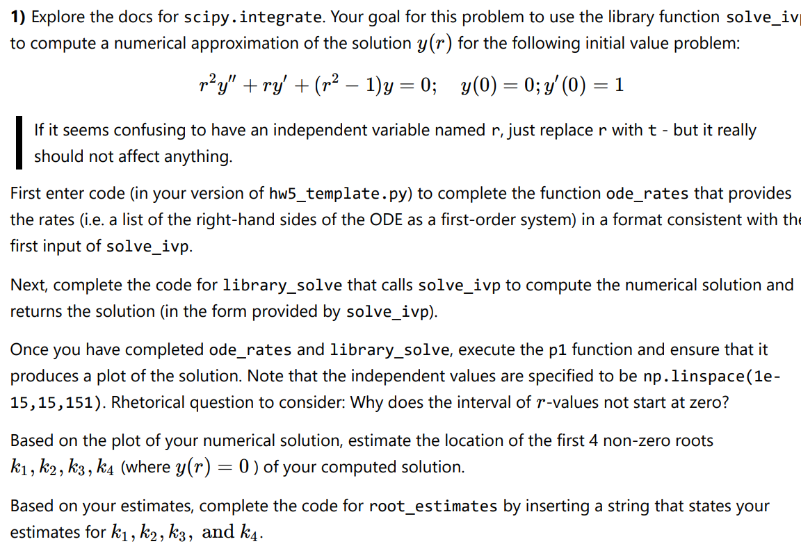
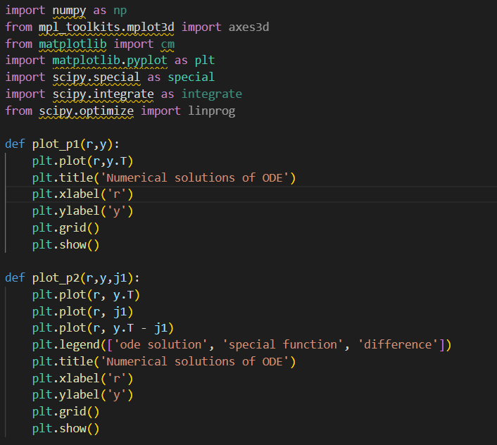
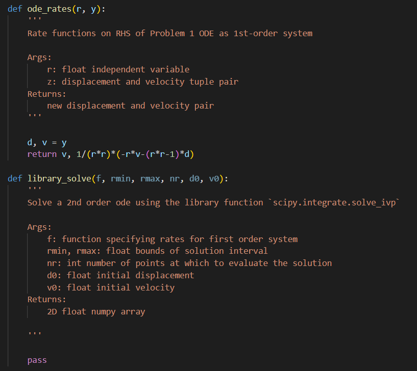
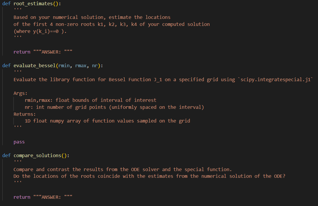
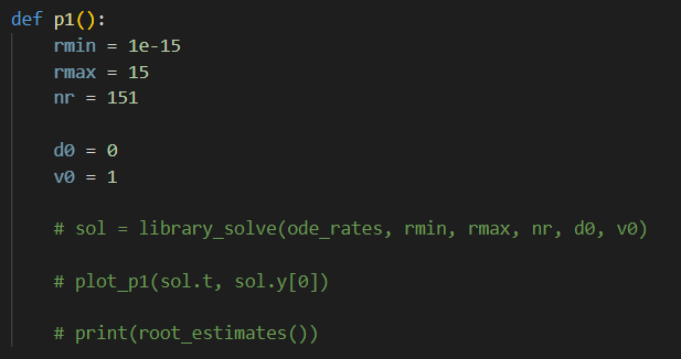
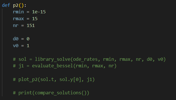
1) Explore the docs for scipy.integrate. Your goal for this problem to use the library function solve_iv to compute a numerical approximation of the solution y(r) for the following initial value problem: r2y+ry+(r21)y=0;y(0)=0;y(0)=1 If it seems confusing to have an independent variable named r, just replace r with t - but it really should not affect anything. First enter code (in your version of hw5_template.py) to complete the function ode_rates that provides the rates (i.e. a list of the right-hand sides of the ODE as a first-order system) in a format consistent with th first input of solve_ivp. Next, complete the code for library_solve that calls solve_ivp to compute the numerical solution and returns the solution (in the form provided by solve_ivp). Once you have completed ode_rates and library_solve, execute the p1 function and ensure that it produces a plot of the solution. Note that the independent values are specified to be np.linspace(1e15,15,151). Rhetorical question to consider: Why does the interval of r-values not start at zero? Based on the plot of your numerical solution, estimate the location of the first 4 non-zero roots k1,k2,k3,k4 (where y(r)=0 ) of your computed solution. Based on your estimates, complete the code for root_estimates by inserting a string that states your 2) Explore the docs for scipy.special. It turns out that the solution to problem 1 is a (fairly) well-known special function: the Bessel function of the first kind of order 1 , a.k.a. J1(r). Find the function that computes the Bessel function J1(r). Fill in code to complete the function evaluate_bessel that returns an array of the special function evaluated on the same array of r values; i.e. np.linspace (1e15,15,151). After completing evaluate_bessel, execute p2() and inspect the plots of the numerical solution, the special function, and the difference between them. 1/3 Then complete compare_solutions by entering a string with your response to the following: "Compare and contrast the results from the ODE solver and the special function. Do the locations of the roots coincide with the estimates from the numerical solution of the ODE?" import numpy as np from mpl toolkits.mplot3d import axes3d from matplotlib import import matplotlib.pyplot as plt import scipy.special as special import scipy.integrate as integrate from scipy.optimize import linprog def plot_p1(r,y): plt.plot(r,y.T) plt.title('Numerical solutions of oDE') plt.xlabel('r') plt.ylabel('y') plt.grid() plt. show() plot_p2(r,y,j1): plt.plot(r, y.T) plt.plot(r, j1) plt.plot(r, y.T - j1) plt.legend(['ode solution', 'special function', 'difference']) plt.title('Numerical solutions of ODE') plt.xlabel('r') plt.ylabel('y') plt.grid() plt.show()