resource code

import numpy as np import matplotlib.pyplot as plt import sympy as sp from scipy.integrate import odeint from scipy.optimize import fsolve import scipy

'''Utilities for MTH 306 in Spring 2019 John Ringland'''

np.seterr(divide='ignore', invalid='ignore')

#%config InlineBackend.figure_format = 'retina' #%matplotlib inline sp.init_printing()

def expressionplot( expression, variable, varmin=0,varmax=1, npts=200, lw=3, alpha=0.5, *args, **kwargs ): '''Plot a sympy expression on specified interval. Sympy itself can do this, but the resulting plot cannot be combined with matplotlib plots (I believe).'''

# When using sp Laplace transform we need to provide a translation for 'Heaviside' that does not exist in numpy def H(z): return 1.*(z>=0) npe = sp.lambdify(variable,expression,['numpy',{'Heaviside':H,'erf':scipy.special.erf}]) npx = np.linspace(varmin,varmax,npts) plt.plot(npx,npe(npx), lw=lw, alpha=alpha, *args, **kwargs)

def get_aspect(ax=None): if ax is None: ax = plt.gca() fig = ax.figure #print( fig.get_size_inches() ) ll, ur = ax.get_position() * fig.get_size_inches() width, height = ur - ll axes_ratio = height / width aspect = axes_ratio / ax.get_data_ratio() return aspect

def slopefieldplot(slopefunction, xlo,xhi, ylo,yhi, yspacing, color='k', lw=3, alpha=0.5, dodots=False, **kwargs): '''Make a slope field plot whose line segments are positioned on a square grid and are all of the same length, regardless of the scales on the horizontal and vertical axes''' # We set the limits first so that the aspect can be determined to allow equal spacing of segment centers in horizontal and vertical directions plt.xlim(xlo,xhi) plt.ylim(ylo,yhi) #print(ax.get_geometry(),ax.get_window_extent(),ax.get_data_ratio(),ax.get_aspect()) a = get_aspect() #print('aspect',a) delta = yspacing tiny = 1.e-6 seghalflengthy = .45 for xc in np.arange(xlo,xhi+np.sign(xhi-xlo)*tiny,a*delta): for yc in np.arange(ylo,yhi+np.sign(yhi-ylo)*tiny,1*delta): if dodots: plt.plot(xc,yc,'o',alpha=0.25,color=color) #angle = np.random.choice([np.pi/2,0]) #np.random.rand()*2*np.pi angle = np.arctan(slopefunction(xc,yc)) c,s = np.cos(angle),np.sin(angle) seghalflength = seghalflengthy*ap.sqrt(c**2 + (a*s)**2) # make all segments the same length on screen dx,dy = c*delta*seghalflength,s*delta*seghalflength plt.plot([xc-dx,xc+dx],[yc-dy,yc+dy],lw=lw,color=color,alpha=0.3)

#def fieldplotlinear(A,xmin,xmax,ymin,ymax,color='b',aspect=None,nx=20,boostarrows=1.,arrowheads=True,alpha=1): # def f(x,y): return np.dot(A,[x,y])[0] # def g(x,y): return np.dot(A,[x,y])[1] # fieldplot(f,g,xmin,xmax,ymin,ymax,color=color,aspect=aspect,nx=nx,boostarrows=boostarrows,arrowheads=arrowheads,alpha=alpha)

def fieldplotlinear(A,xmin,xmax,ymin,ymax,color='b',aspect=None,nx=20,boostarrows=1.,arrowheads=True,alpha=1): def F(X): return np.dot(A,X) fieldplot(F,xmin,xmax,ymin,ymax,color=color,aspect=aspect,nx=nx,boostarrows=boostarrows,arrowheads=arrowheads,alpha=alpha)

def fieldplot2(f,g,xmin,xmax,ymin,ymax,color='b',aspect=None,nx=20,boostarrows=1.,arrowheads=True,alpha=1): '''f and g are numpy-friendly functions of 2 variables''' #plt.clf() #figure(figsize=(12,12)) #figure(figsize=(8,8),facecolor='w') #nx = 20 xr = xmax-xmin yr = ymax-ymin ny = int(nx*yr/xr) if aspect!=None: plt.subplot(111,aspect=aspect) X,Y = np.meshgrid( np.linspace(xmin,xmax,nx), np.linspace(ymin,ymax,ny) ) X = X.flatten() Y = Y.flatten() U = f(X,Y) V = g(X,Y) #print(U) #print(V) # scale length of arrows - note arrowhead is added beyond the end of the line segment h = boostarrows*0.9*min(xr/float(nx-1)/abs(U).max(),yr/float(ny-1)/abs(V).max()) Xp = X + h*U Yp = Y + h*V arrowsX = np.vstack((X,Xp)) arrowsY = np.vstack((Y,Yp)) if arrowheads: head_width = 0.005*xr else: head_width = 0 head_length = head_width/0.6

for xc,yc,u,v in zip(X,Y,U,V): plt.arrow( xc,yc, h*u,h*v, fc=color, ec=color, alpha=alpha, width=head_width/5, head_width=head_width, head_length=head_length ) plt.xlim(xmin,xmax) # plot ranges strangely are [0,1] x [0,1] otherwise plt.ylim(ymin,ymax) def fieldplot(F,xmin,xmax,ymin,ymax,color='b',aspect=None,nx=20,boostarrows=1.,arrowheads=True,alpha=1): def f(x,y): return F((x,y))[0] def g(x,y): return F((x,y))[1] # Doing it this way is unfortunately twice the work (2 calls to F for every evaluation) '''f and g are numpy-friendly functions of 2 variables''' #plt.clf() #figure(figsize=(12,12)) #figure(figsize=(8,8),facecolor='w') #nx = 20 xr = xmax-xmin yr = ymax-ymin ny = int(nx*yr/xr) if aspect!=None: plt.subplot(111,aspect=aspect) X,Y = np.meshgrid( np.linspace(xmin,xmax,nx), np.linspace(ymin,ymax,ny) ) X = X.flatten() Y = Y.flatten() U = f(X,Y) V = g(X,Y) #print(U) #print(V) # scale length of arrows - note arrowhead is added beyond the end of the line segment h = boostarrows*0.9*min(xr/float(nx-1)/abs(U).max(),yr/float(ny-1)/abs(V).max()) Xp = X + h*U Yp = Y + h*V arrowsX = np.vstack((X,Xp)) arrowsY = np.vstack((Y,Yp)) if arrowheads: head_width = 0.005*xr else: head_width = 0 head_length = head_width/0.6

for xc,yc,u,v in zip(X,Y,U,V): plt.arrow( xc,yc, h*u,h*v, fc=color, ec=color, alpha=alpha, width=head_width/5, head_width=head_width, head_length=head_length ) plt.xlim(xmin,xmax) # plot ranges strangely are [0,1] x [0,1] otherwise plt.ylim(ymin,ymax)

def phaseportrait(F,ics=[], *args, **kwargs): # F is a vector-valued function of a vector argument #print(kwargs) def FF(X,t): return F(X) # odeint allows non-autonomous system for ict in ics: ic = ict[:2] if len(ict)==3: # initial time as 0 and 3rd argument as final time t1s = [ict[2]] elif len(ict)==4: t1s = [ict[2],ict[3]] else: t1s = [10] # default final time for t1 in t1s: t = np.linspace(0,t1,500) Y = odeint(FF,ic,t) plt.plot(Y[:,0],Y[:,1],*args, **kwargs)

#def phaseportraitlinear(A,ics=[], *args, **kwargs): # A is a sympy or numpy matrix # #print(kwargs) # Af = np.array(A,dtype=float) # def f(x,y): return Af[0,0]*x + Af[0,1]*y # def g(x,y): return Af[1,0]*x + Af[1,1]*y # def F(X): # version of f,g with vector input and output # x,y = X # return f(x,y),g(x,y) # fieldplot(f,g,-1,1,-1,1,color='k',alpha=0.25) # phaseportrait(F, ics, *args, **kwargs) def phaseportraitlinear(A,ics=[], *args, **kwargs): # A is a sympy or numpy matrix #print(kwargs) Af = np.array(A,dtype=float) def F(X): # version of f,g with vector input and output return np.dot(Af,X) fieldplot(F,-1,1,-1,1,color='k',alpha=0.25) phaseportrait(F, ics, *args, **kwargs)

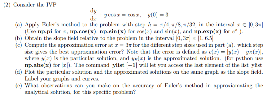
(2) Consider the IVP + y cos I = cosr, y(0) = 3 (a) Apply Euler's method to the problem with step h = 7/4, 7/8, 7/32, in the interval - 0,37] (Use np.pi for a, np.cos(x), np.sin(x) for cos(2) and sin(2), and np.exp(x) for et ). (b) Obtain the slope field relative to the problem in the interval (0,37 x 1, 6.5 (c) Compute the approximation error at r = 37 for the different step sizes used in part (a). which step size gives the best approximation error? Note that the error is defined as e(r) = ly(c)-YEC), where y ) is the particular solution, and ye 2) is the approximated solution. (for python use np.abs(x) for xD). The command ylist (-1) will let you access the last element of the list ylist (d) Plot the particular solution and the approximated solutions on the same graph as the slope field. Label your graphs and curves. (e) What observations can you make on the accuracy of Euler's method in approxiamating the analytical solution, for this specific problem? (2) Consider the IVP + y cos I = cosr, y(0) = 3 (a) Apply Euler's method to the problem with step h = 7/4, 7/8, 7/32, in the interval - 0,37] (Use np.pi for a, np.cos(x), np.sin(x) for cos(2) and sin(2), and np.exp(x) for et ). (b) Obtain the slope field relative to the problem in the interval (0,37 x 1, 6.5 (c) Compute the approximation error at r = 37 for the different step sizes used in part (a). which step size gives the best approximation error? Note that the error is defined as e(r) = ly(c)-YEC), where y ) is the particular solution, and ye 2) is the approximated solution. (for python use np.abs(x) for xD). The command ylist (-1) will let you access the last element of the list ylist (d) Plot the particular solution and the approximated solutions on the same graph as the slope field. Label your graphs and curves. (e) What observations can you make on the accuracy of Euler's method in approxiamating the analytical solution, for this specific