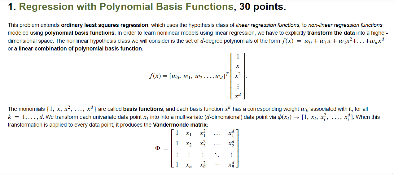
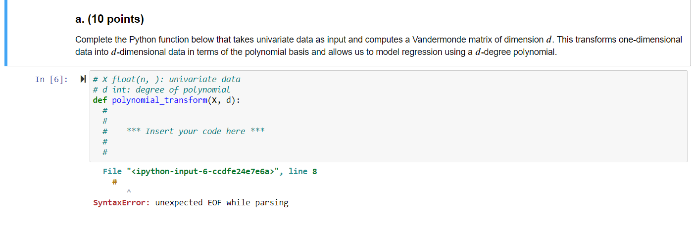
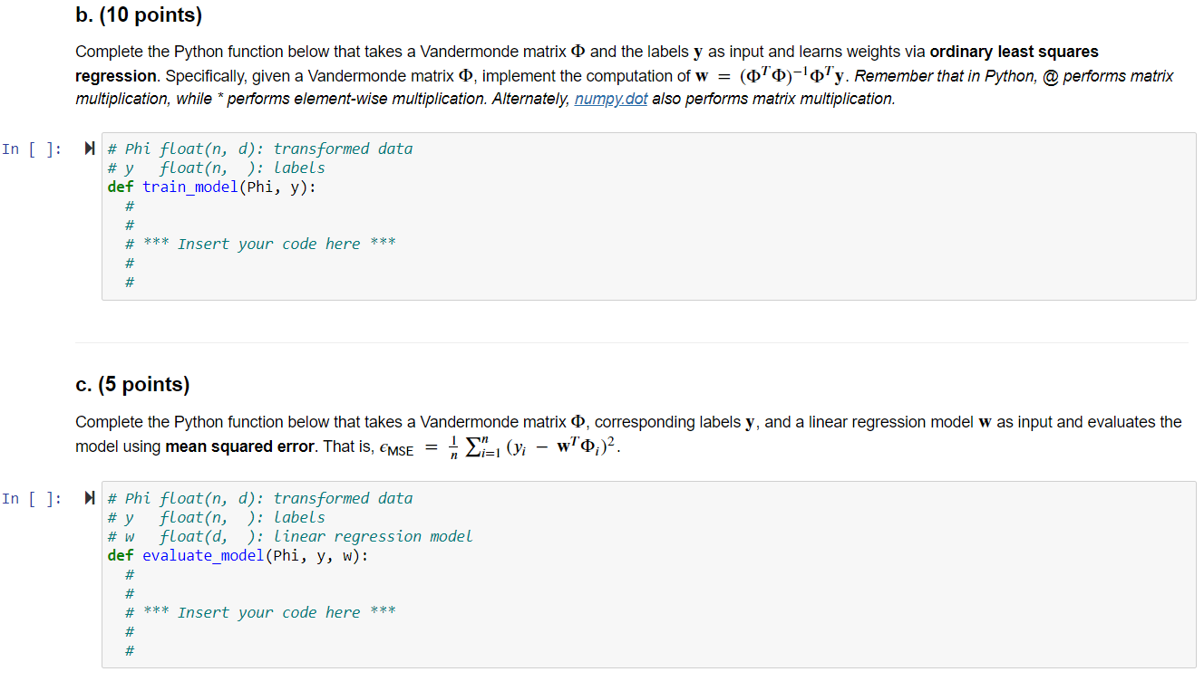
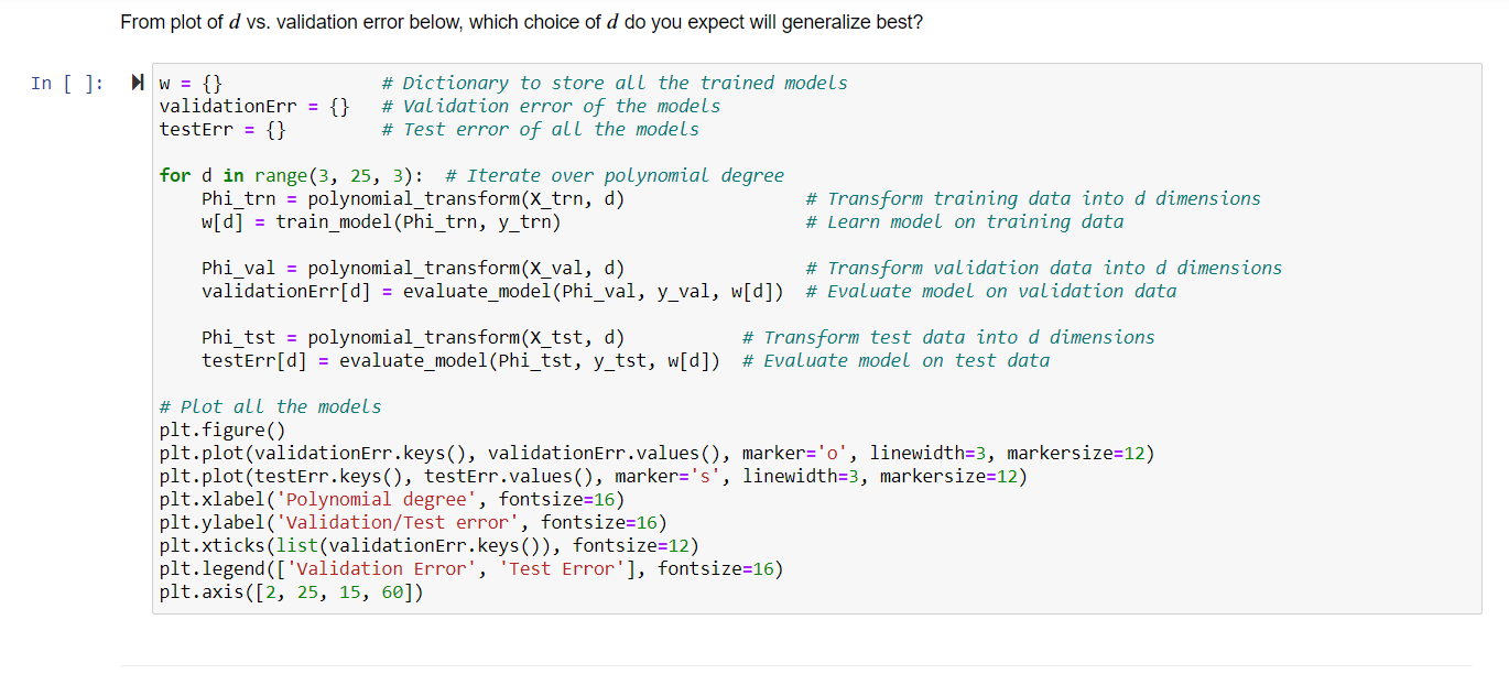
1. Regression with Polynomial Basis Functions, 30 points. This problem extends ordinary least squares regression, which uses the hypothesis class of linear regression functions, to non-linear regression functions modeled using polynomial basis functions. In order to learn nonlinear models using linear regression, we have to explicitly transform the data into a higher- dimensional space. The nonlinear hypothesis class we will consider is the set of d-degree polynomials of the form f(x) = wo + w1x + w2x+...+wqxd or a linear combination of polynomial basis function: X f(x) = [wo, W1, W2 ..., wa] x2 rd The monomials {1, x, x, ..., xd } are called basis functions, and each basis function xk has a corresponding weight wk associated with it, for all k = 1,..., d. We transform each univariate data point x; into into a multivariate (d-dimensional) data point via p(x;) [1, x, xz, x]. When this transformation is applied to every data point, it produces the Vandermonde matrix: X1 x? 1 x2 x? : : 0 = 1 xn a. (10 points) Complete the Python function below that takes univariate data as input and computes a Vandermonde matrix of dimension d. This transforms one-dimensional data into d-dimensional data in terms of the polynomial basis and allows us to model regression using a d-degree polynomial. In [6]: # x float(n, ): univariate data # d int: degree of polynomial def polynomial_transform(x, d): # # # *** Insert your code here *** # # File "", line 8 SyntaxError: unexpected EOF while parsing b. (10 points) Complete the Python function below that takes a Vandermonde matrix o and the labels y as input and learns weights via ordinary least squares regression. Specifically, given a Vandermonde matrix O, implement the computation of w = (070)-'0'y. Remember that in Python, @performs matrix multiplication, while * performs element-wise multiplication. Alternately, numpy.dot also performs matrix multiplication. In [ ]: # Phi float(n, d): transformed data # y float(n, ): Labels def train_model(Phi, y): # # # *** Insert your code here *** # # c. (5 points) Complete the Python function below that takes a Vandermonde matrix o, corresponding labels y, and a linear regression model w as input and evaluates the model using mean squared error. That is, emse = X= (yi wo;) In [ ]: # Phi float(n, d): transformed data # y float(n, ): Labels float(d, ): Linear regression model def evaluate_model(Phi, y, w): # w # # # *** Insert your code here *** # # From plot of d vs. validation error below, which choice of d do you expect will generalize best? In [ ]: W = {} validationErr = testErr = {} {} # Dictionary to store all the trained models # Validation error of the models # Test error of all the models for d in range(3, 25, 3): # Iterate over polynomial degree Phi_trn = polynomial_transform(x_trn, d) w[d] = train_model(Phi_trn, y tnn) # Transform training data into d dimensions # Learn model on training data Phi_val = polynomial_transform(X_val, d) # Transform validation data into d dimensions validationErr[d] = evaluate_model(Phi_val, y_val, w[d]) # Evaluate model on validation data Phi_tst = polynomial_transform(x_tst, d) # Transform test data into d dimensions testErr[d] = evaluate_model(Phi_tst, y_tst, w[d]) # Evaluate model on test data # Plot all the models plt.figure() plt.plot(validationErr.keys(), validationErr.values(), marker='o', linewidth=3, markersize=12) plt.plot(testErr.keys(), testErr.values(), marker='s', linewidth=3, markersize=12) plt.xlabel('Polynomial degree', fontsize=16) plt.ylabel('Validation/Test error', fontsize=16) plt.xticks (list(validationErr.keys()), fontsize=12) plt.legend (['Validation Error', 'Test Error'], fontsize=16) plt.axis ([2, 25, 15, 60]) 1. Regression with Polynomial Basis Functions, 30 points. This problem extends ordinary least squares regression, which uses the hypothesis class of linear regression functions, to non-linear regression functions modeled using polynomial basis functions. In order to learn nonlinear models using linear regression, we have to explicitly transform the data into a higher- dimensional space. The nonlinear hypothesis class we will consider is the set of d-degree polynomials of the form f(x) = wo + w1x + w2x+...+wqxd or a linear combination of polynomial basis function: X f(x) = [wo, W1, W2 ..., wa] x2 rd The monomials {1, x, x, ..., xd } are called basis functions, and each basis function xk has a corresponding weight wk associated with it, for all k = 1,..., d. We transform each univariate data point x; into into a multivariate (d-dimensional) data point via p(x;) [1, x, xz, x]. When this transformation is applied to every data point, it produces the Vandermonde matrix: X1 x? 1 x2 x? : : 0 = 1 xn a. (10 points) Complete the Python function below that takes univariate data as input and computes a Vandermonde matrix of dimension d. This transforms one-dimensional data into d-dimensional data in terms of the polynomial basis and allows us to model regression using a d-degree polynomial. In [6]: # x float(n, ): univariate data # d int: degree of polynomial def polynomial_transform(x, d): # # # *** Insert your code here *** # # File "", line 8 SyntaxError: unexpected EOF while parsing b. (10 points) Complete the Python function below that takes a Vandermonde matrix o and the labels y as input and learns weights via ordinary least squares regression. Specifically, given a Vandermonde matrix O, implement the computation of w = (070)-'0'y. Remember that in Python, @performs matrix multiplication, while * performs element-wise multiplication. Alternately, numpy.dot also performs matrix multiplication. In [ ]: # Phi float(n, d): transformed data # y float(n, ): Labels def train_model(Phi, y): # # # *** Insert your code here *** # # c. (5 points) Complete the Python function below that takes a Vandermonde matrix o, corresponding labels y, and a linear regression model w as input and evaluates the model using mean squared error. That is, emse = X= (yi wo;) In [ ]: # Phi float(n, d): transformed data # y float(n, ): Labels float(d, ): Linear regression model def evaluate_model(Phi, y, w): # w # # # *** Insert your code here *** # # From plot of d vs. validation error below, which choice of d do you expect will generalize best? In [ ]: W = {} validationErr = testErr = {} {} # Dictionary to store all the trained models # Validation error of the models # Test error of all the models for d in range(3, 25, 3): # Iterate over polynomial degree Phi_trn = polynomial_transform(x_trn, d) w[d] = train_model(Phi_trn, y tnn) # Transform training data into d dimensions # Learn model on training data Phi_val = polynomial_transform(X_val, d) # Transform validation data into d dimensions validationErr[d] = evaluate_model(Phi_val, y_val, w[d]) # Evaluate model on validation data Phi_tst = polynomial_transform(x_tst, d) # Transform test data into d dimensions testErr[d] = evaluate_model(Phi_tst, y_tst, w[d]) # Evaluate model on test data # Plot all the models plt.figure() plt.plot(validationErr.keys(), validationErr.values(), marker='o', linewidth=3, markersize=12) plt.plot(testErr.keys(), testErr.values(), marker='s', linewidth=3, markersize=12) plt.xlabel('Polynomial degree', fontsize=16) plt.ylabel('Validation/Test error', fontsize=16) plt.xticks (list(validationErr.keys()), fontsize=12) plt.legend (['Validation Error', 'Test Error'], fontsize=16) plt.axis ([2, 25, 15, 60])