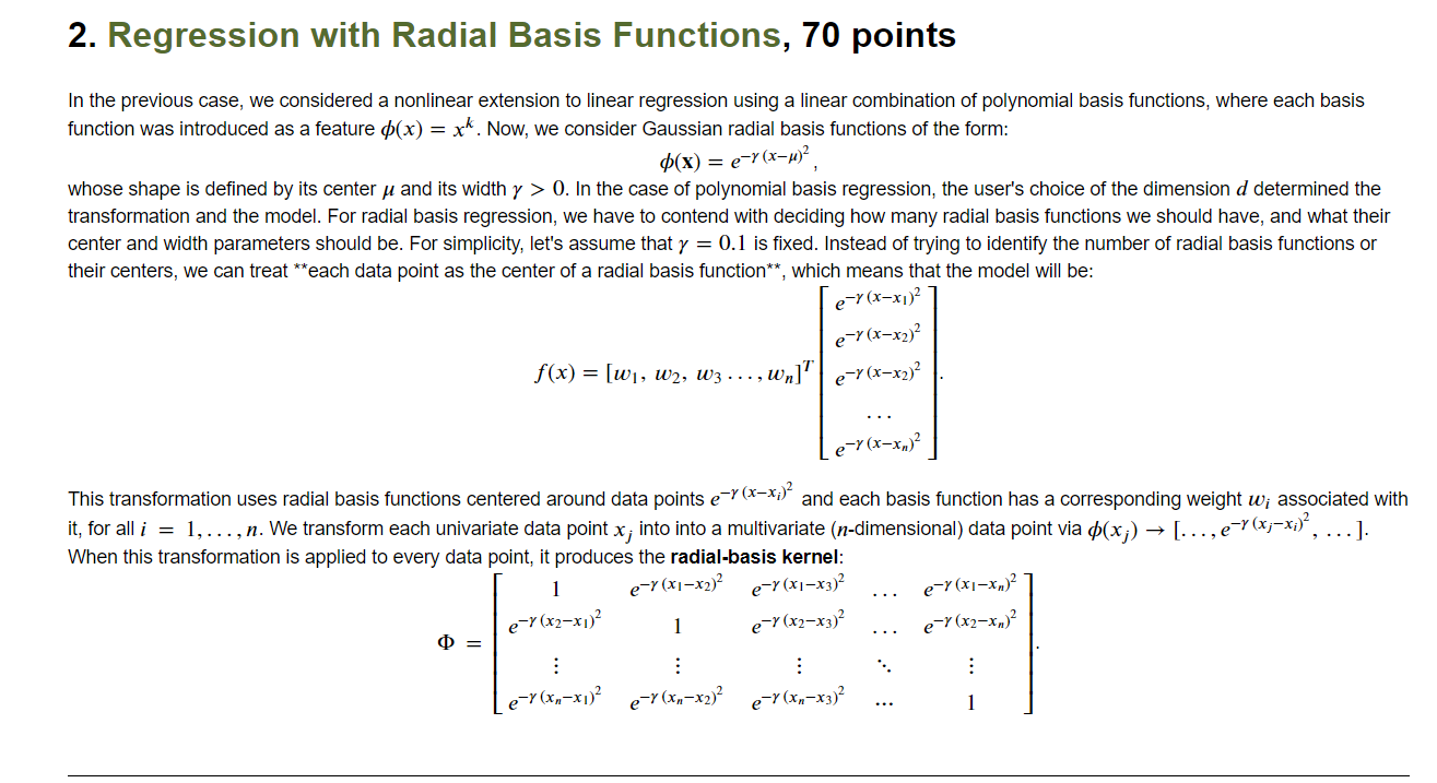
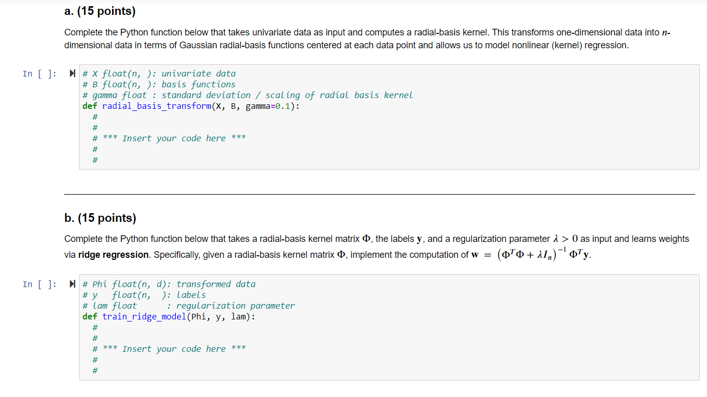
2. Regression with Radial Basis Functions, 70 points In the previous case, we considered a nonlinear extension to linear regression using a linear combination of polynomial basis functions, where each basis function was introduced as a feature P(x) = xk. Now, we consider Gaussian radial basis functions of the form: $(x) = e-Y(x-4)2 whose shape is defined by its center u and its width y > 0. In the case of polynomial basis regression, the user's choice of the dimension d determined the transformation and the model. For radial basis regression, we have to contend with deciding how many radial basis functions we should have, and what their center and width parameters should be. For simplicity, let's assume that y = 0.1 is fixed. Instead of trying to identify the number of radial basis functions or their centers, we can treat **each data point as the center of a radial basis function**, which means that the model will be: e-y(x-x1) e-Y(x-x2) f(x) = [w], W2, W3 ..., wn]"e-(x-x2)2 le=(x-xw)2 This transformation uses radial basis functions centered around data points e-Y(x=x;)? and each basis function has a corresponding weight w; associated with it, for all i = 1,..., n. We transform each univariate data point x; into into a multivariate (n-dimensional) data point via $(x;) [..., e(x;=x;), ...). When this transformation is applied to every data point, it produces the radial-basis kernel: 1 e-> (x1-x2)2 e-Y(x1-x3)2 e-Y(x2-x]) e-Y(x2-x3)2 e-Y(x2-x.,) : : : e-Y(x,-x1) e->(x,-x2) e-Y(x2-x3)? 1 e-Y(x1-x)2 a. (15 points) Complete the Python function below that takes univariate data as input and computes a radial-basis kernel. This transforms one-dimensional data into n- dimensional data in terms of Gaussian radial-basis functions centered at each data point and allows us to model nonlinear (kernel) regression. In [ ]: # X float(n, ): univariate data # B float(n, ): basis functions # gamma float : standard deviation / scaling of radial basis kernel def radial_basis_transform(X, B, gamma=0.1): # # # *** Insert your code here *** # # b. (15 points) Complete the Python function below that takes a radial-basis kernel matrix o, the labels y, and a regularization parameter 1 > 0 as input and learns weights via ridge regression. Specifically, given a radial-basis kernel matrix o, implement the computation of w = (oo + 11,)-'oy In [ ]: # Phi float(n, d): transformed data # y float(n, ): Labels # Lam float i regularization parameter def train_ridge_model(Phi, y, lam): # # # *** Insert your code here *** # # c. (30 points) As before, we can explore the tradeoff between fit and complexity by varying a [10-3, 10-2 ..., 1, ... 103]. For each model, train using the transformed training data (0) and evaluate its performance on the transformed validation and test data. Plot two curves: (i) a vs. validation error and (ii) a vs. test error, as above. What are some ideal values of 1? In [ ]: # # *** Insert your code here *** # d. (10 points, Discussion) Plot the learned models as well as the true model similar to the polynomial basis case above. How does the linearity of the model change with 2? In [ ]: # # *** Insert your code here *** 2. Regression with Radial Basis Functions, 70 points In the previous case, we considered a nonlinear extension to linear regression using a linear combination of polynomial basis functions, where each basis function was introduced as a feature P(x) = xk. Now, we consider Gaussian radial basis functions of the form: $(x) = e-Y(x-4)2 whose shape is defined by its center u and its width y > 0. In the case of polynomial basis regression, the user's choice of the dimension d determined the transformation and the model. For radial basis regression, we have to contend with deciding how many radial basis functions we should have, and what their center and width parameters should be. For simplicity, let's assume that y = 0.1 is fixed. Instead of trying to identify the number of radial basis functions or their centers, we can treat **each data point as the center of a radial basis function**, which means that the model will be: e-y(x-x1) e-Y(x-x2) f(x) = [w], W2, W3 ..., wn]"e-(x-x2)2 le=(x-xw)2 This transformation uses radial basis functions centered around data points e-Y(x=x;)? and each basis function has a corresponding weight w; associated with it, for all i = 1,..., n. We transform each univariate data point x; into into a multivariate (n-dimensional) data point via $(x;) [..., e(x;=x;), ...). When this transformation is applied to every data point, it produces the radial-basis kernel: 1 e-> (x1-x2)2 e-Y(x1-x3)2 e-Y(x2-x]) e-Y(x2-x3)2 e-Y(x2-x.,) : : : e-Y(x,-x1) e->(x,-x2) e-Y(x2-x3)? 1 e-Y(x1-x)2 a. (15 points) Complete the Python function below that takes univariate data as input and computes a radial-basis kernel. This transforms one-dimensional data into n- dimensional data in terms of Gaussian radial-basis functions centered at each data point and allows us to model nonlinear (kernel) regression. In [ ]: # X float(n, ): univariate data # B float(n, ): basis functions # gamma float : standard deviation / scaling of radial basis kernel def radial_basis_transform(X, B, gamma=0.1): # # # *** Insert your code here *** # # b. (15 points) Complete the Python function below that takes a radial-basis kernel matrix o, the labels y, and a regularization parameter 1 > 0 as input and learns weights via ridge regression. Specifically, given a radial-basis kernel matrix o, implement the computation of w = (oo + 11,)-'oy In [ ]: # Phi float(n, d): transformed data # y float(n, ): Labels # Lam float i regularization parameter def train_ridge_model(Phi, y, lam): # # # *** Insert your code here *** # # c. (30 points) As before, we can explore the tradeoff between fit and complexity by varying a [10-3, 10-2 ..., 1, ... 103]. For each model, train using the transformed training data (0) and evaluate its performance on the transformed validation and test data. Plot two curves: (i) a vs. validation error and (ii) a vs. test error, as above. What are some ideal values of 1? In [ ]: # # *** Insert your code here *** # d. (10 points, Discussion) Plot the learned models as well as the true model similar to the polynomial basis case above. How does the linearity of the model change with 2? In [ ]: # # *** Insert your code here ***