10.2 Fitting a Linear Model To Data.

Answer All of the questions and SHOW YOUR WORK!

Explore 1: Plotting and Analyzing Residuals questions A, B, C, D, Reflect 1 and 2. SHOW YOUR WORK!

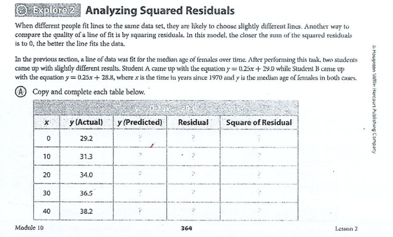
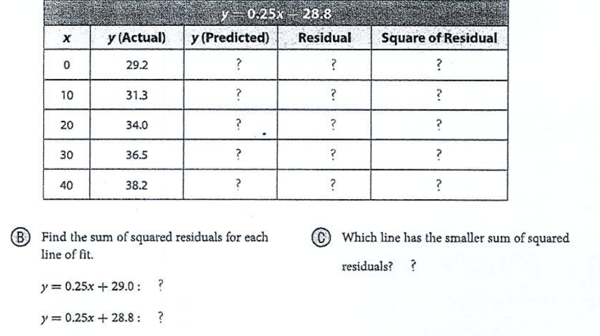
Explore 2: Analyzing Squared Residuals questions A, B, C, and Reflect 3 and 4. SHOW YOUR WORK!

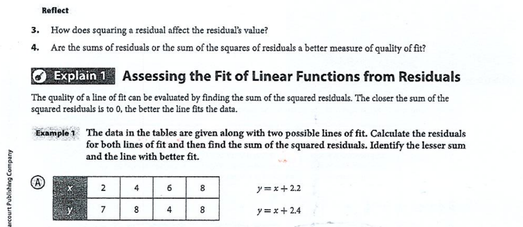
Explain 1: Assessing the Fit of Linear Functions from Residuals Example 1 Questions A, a, B, b, a, b, Reflect 5, 6, and 7. SHOW YOUR WORK!

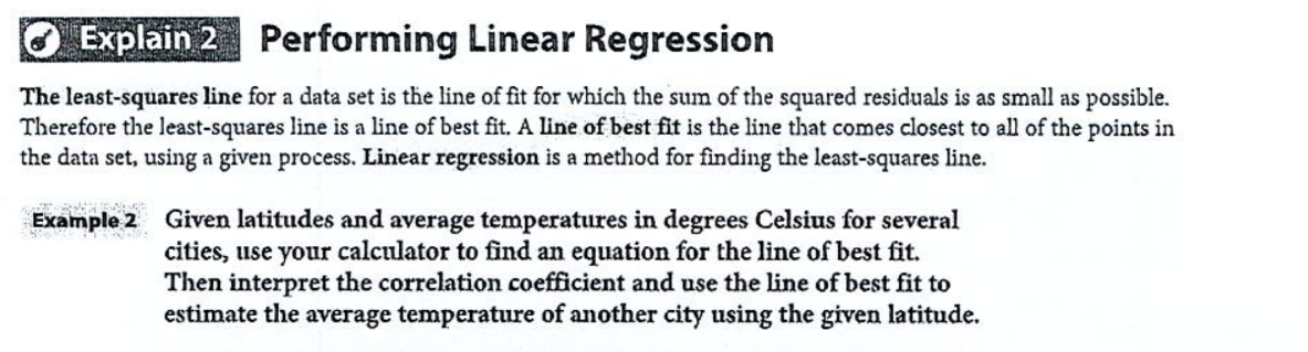
Explain 2: Performing Linear Regression Example 2 answer questions A, B, Reflect 8 and 9. SHOW YOUR WORK!

The information Reference is from: Houghton Mifflin Harcourt Publishing Company.

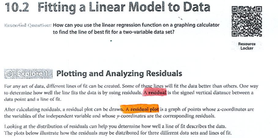
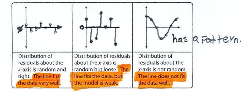
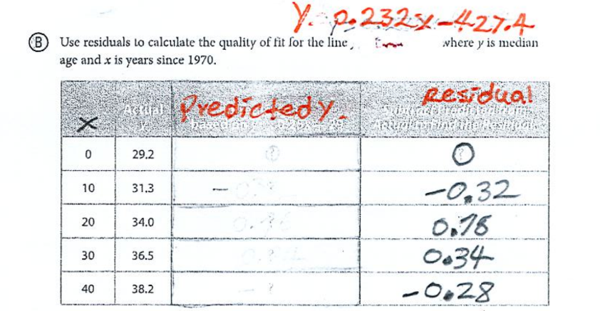
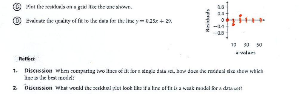
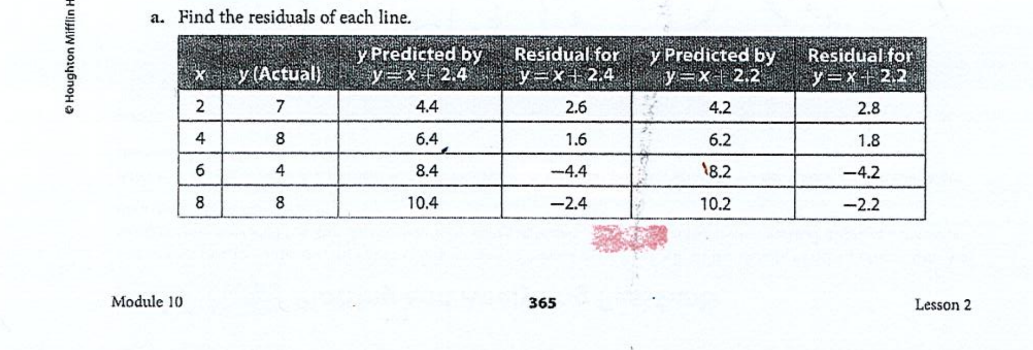
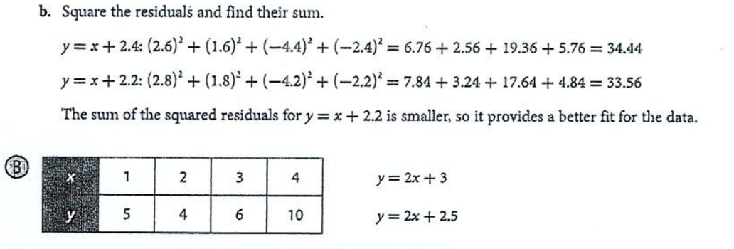
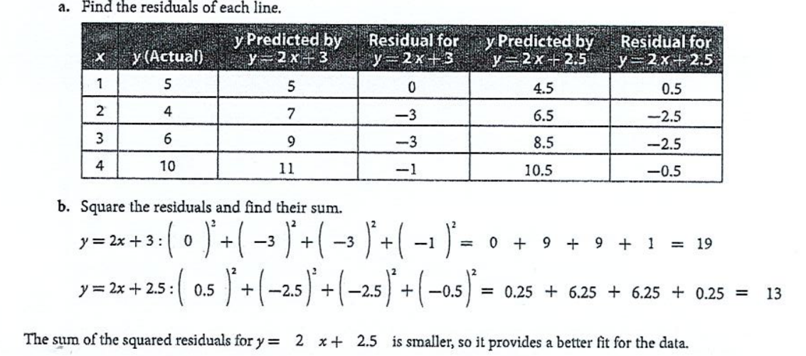
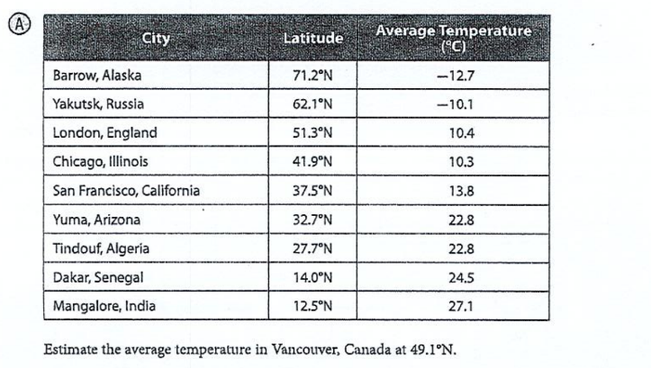
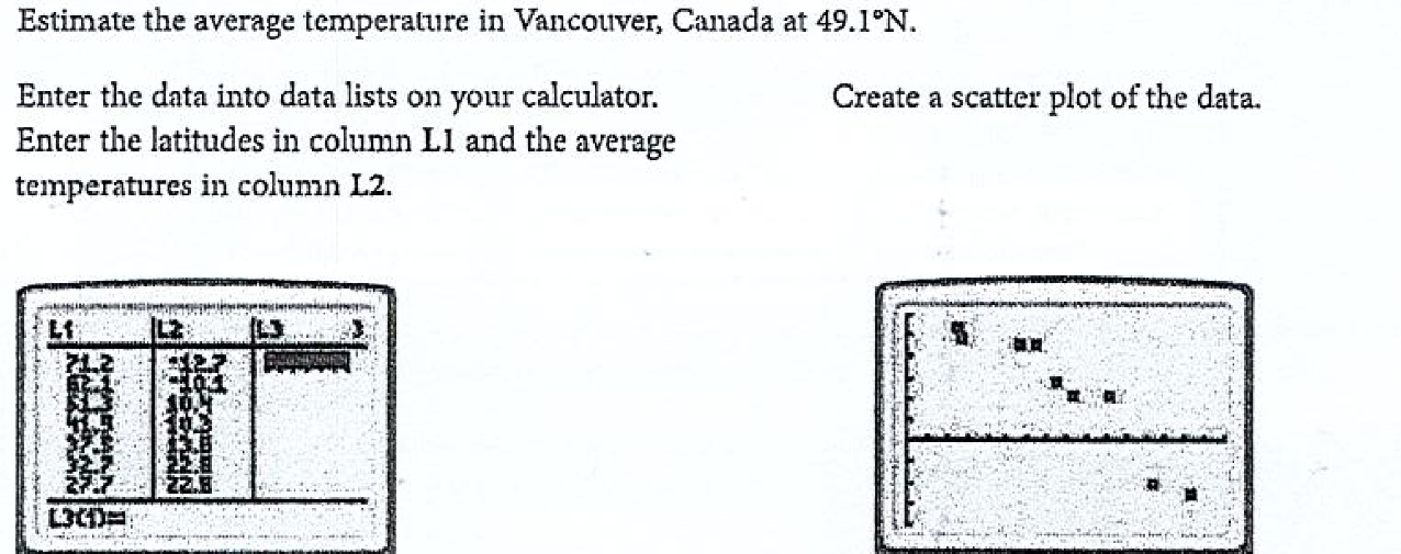
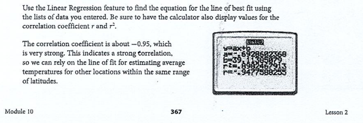
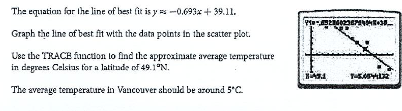
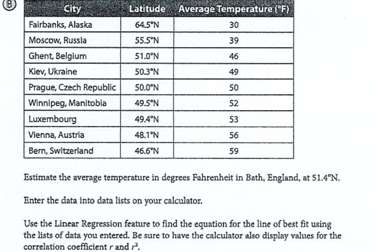
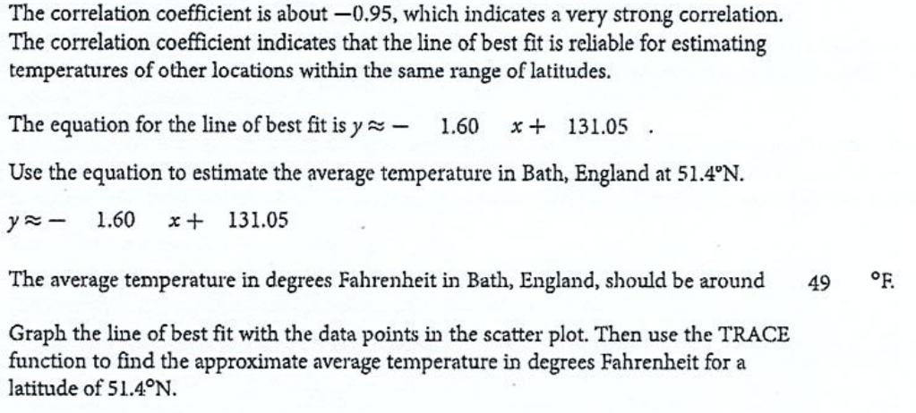
10.2 Fitting a Linear Model to Data Essential Question: How can you use the linear regression function on a graphing calculator to find the line of best fit for a two-variable data set? Resource Locker Plotting and Analyzing Residuals For any set of data, different lines of fit can be created. Some of these lines will fit the data better than others. One way to determine how well the line fits the data is by using residuals. A residual is the signed vertical distance between a data point and a line of fit. After calculating residuals, a residual plot can be drawn. A residual plot is a graph of points whose x-coordinates are the variables of the independent variable and whose y-coordinates are the corresponding residuals. Looking at the distribution of residuals can help you determine how well a line of fit describes the data. The plots below illustrate how the residuals may be distributed for three different data sets and lines of fit.O has a pattern. Distribution of Distribution of residuals Distribution of residuals about the about the x-axis is residuals about the x-axis is random and random but loose. The x-axis is not random. tight. The line fits line fits the data, but The line does not fit the data very well. the model is weak. the data well.The table lists the median age of females living in the United States, based on the results of the United States Census over the past few decades. Follow the steps listed to complete the task. A Use the table to create a table of paired values for x and y. Let x represent the time in years after 1970 and y represent the median age of females. " Houghton Mifflin Harcourt Publishing Company . In bikeriderlondon/Shutterstock 1970 29.2 1980 31.3 1990 34.0 2000 36.5 2010 38.2 Module 10 363 Lesson 2Y. p.232x-427.4 B Use residuals to calculate the quality of fit for the line , where y is median age and x is years since 1970. Predictedy Residual X 0 29.2 10 31.3 -0.32 20 34.0 30 36.5 0 0 34 40 38.2 - 0.28Plot the residuals on a grid like the one shown. 0.8 0.4 D Evaluate the quality of fit to the data for the line y = 0.25x +- 29. Residuals 0 -0.4 -0.8 10 30 50 x-values Reflect 1. Discussion When comparing two lines of fit for a single data set, how does the residual size show which line is the best model? 2. Discussion What would the residual plot look like if a line of fit is a weak model for a data set?Explore 2 Analyzing Squared Residuals When different people fit lines to the same data set, they are likely to choose slightly different lines. Another way to compare the quality of a line of fit is by squaring residuals. In this model, the closer the sum of the squared residuals is to 0, the better the line fits the data. In the previous section, a line of data was fit for the median age of females over time. After performing this task, two students came up with slightly different results. Student A come up with the equation y = 0.25x + 29.0 while Student B came up with the equation y = 0.25x + 28.8, where x is the time in years since 1970 and y is the median age of females in both cases. Copy and complete each table below. X y (Actual) y (Predicted) Residual Square of Residual 0 29.2 10 31.3 20 34.0 30 36.5 40 38.2 Module 10 364 Lesson 2v 0125;: 23 3 Find the sum of squared residuals for each Which line has the smaller sum of squared line of fit. residuals? y=025x+290: y=025x+288: ? arcourt Publishing Company 3. How does squaring a residual affect the residual's value? 4. Arc the sums of residuals or the sum of the squares of residuals a better measure of quality of fit? Assessing the Fit of Linear Functions from Residuals The quality of a line of fit can be evaluated by finding the sum of the squared residuals. The closer the sum of the squared residuals is to 0, the better the line fits the data. Example 1 The data in the tables are given along with two possible lines of fit. Calculate the residuals ~ for both lines of fit and then find the sum of the squared residuals. Identify the lesser sum and the line with better fit. @ a. Find the residuals of each line. Houghton Mifflin y Predicted by Residual for y Predicted by Residual for y (Actual) V -X + 2.4 =X 1 2.4 Y X | 2.2 y = X + 2.2 2 7 4.4 2.6 4.2 2.8 4 6.4 1.6 6.2 1.8 6 4 8.4 -4.4 18.2 -4.2 8 10.4 -2.4 10.2 -2.2 Module 10 365 Lesson 2b. Square the residuals and find their sum. y=x+ 2.4:(2.6)" + (1.6)* + (4.4)" + (2.4)" = 6.76 + 2.56 + 19.36 + 5.76 = 34.44 y=x+22:(2.8)" + (1.8) + (4.2) + (2.2)* = 7.84 + 3.24 + 17.64 + 4.84 = 33.56 The sum of the squared residuals for y = x + 2.2 is smaller, so it provides a better fit for the data. a. Find the residuals of each line. y Predicted by Residual for _y Predicted by Residual for y (Actual) Y 2x +3 y -2x LB Y -2x - 2.5 y -2x + 2.5 1 5 UT 0 4.5 0.5 2 4 7 6.5 -2.5 3 6 9 8.5 -2.5 4 10 11 -1 10.5 -0.5 b. Square the residuals and find their sum. y = 2x + 3 : 0 + -3 + -3 +-1 =0+ 9+ 9+ 1 = 19 y = 2x + 2.5: 0.5 + -2.5 +-2.5+-0.5)= 0.25 + 6.25 + 6.25 + 0.25 = 13 The sum of the squared residuals for y = 2 x + 2.5 is smaller, so it provides a better fit for the data.Reflect 5. How do negative signs on residuals affect the sum of squared residuals? 6. Why do small values for residuals mean that a line of best fit has a tight fit to the data? Your Turn 7. The data in the table are given along with two possible lines of fit. Calculate the residuals for both lines of fit and then find the sum of the squared residuals. Identify the lesser sum and the line with better fit. 2 3 4 y=X+4 @ Houghton Mifflin Harcourt Publishing Company 4 7 8 6 y = x + 4.2 Module 10 366 Lesson 2(o W'GIETL B Performing Linear Regression The least-squares line for a data set is the line of fit for which the sum of the squared residuals is as small as possible. Therefore the least-squares line is a line of best fit. A line of best fit is the line that comes closest to all of the points in the data set, using a given process. Linear regression is a method for finding the least-squares line. 'Example2 Given latitudes and average temperatures in degrees Celsius for several cities, use your calculator to find an equation for the line of best fit. Then interpret the correlation coefficient and use the line of best fit to estimate the average temperature of another city using the given latitude. City Latitude Average Temperature (SC) Barrow, Alaska 71.2'N -12.7 Yakutsk, Russia 62.1'N -10.1 London, England 51.3'N 10.4 Chicago, Illinois 41.9'N 10.3 San Francisco, California 37.5'N 13.8 Yuma, Arizona 32.7'N 22.8 Tindouf, Algeria 27.7'N 22.8 Dakar, Senegal 14.0'N 24.5 Mangalore, India 12.5'N 27.1 Estimate the average temperature in Vancouver, Canada at 49.1"N.Estimate the average temperature in Vancouver, Canada at 49.1 N. Enter the data into data lists on your calculator. Create a scatter plot of the data. Enter the latitudes in column LI and the average temperatures in column L2.Use the Linear Regression feature to find the equation for the line of best fit using the lists of data you entered. Be sure to have the calculator also display values for the correlation coefficient rand r, The correlation coefficient is about 0.95, which is very strong. This indicates a strong orrelation, so we can rely on the line of fit for estimating average temperatures for other locations within the same range of latitudes. Module 10 367 . Lesson 2 The equation for the line of best [it is y = 0.693x + 39.11. Graph the line of best fit with the data points in the scatter plot. Use the TRACE function to find the approximate average temperature in degrees Celsius for a latitude of 49.1N. : The average temperature in Vancouver should be around 5C. B City Latitude Average Temperature ( F) Fairbanks, Alaska 64.5'N 30 Moscow, Russia 55.5"N 39 Ghent, Belgium 51.0'N 46 Kiev, Ukraine 50.3'N 49 Prague, Czech Republic 50.0 N 50 Winnipeg, Manitobia 49.5'N 52 Luxembourg 49.4'N 53 Vienna, Austria 48.1'N 56 Bern, Switzerland 46.6'N 59 Estimate the average temperature in degrees Fahrenheit in Bath, England, at 51.4"N. Enter the data into data lists on your calculator. Use the Linear Regression feature to find the equation for the line of best fit using the lists of data you entered. Be sure to have the calculator also display values for the correlation coefficient r and r?.The correlation coefficient is about 0.95, which indicates a very strong correlation. The correlation coefficient indicates that the line of best fit is reliable for estimating temperatures of other locations within the same range of latitudes. The equation for the line of best fitisy~ 1,60 x+ 131.05 Use the equation to estimate the average temperature in Bath, England at 51.4N. y~ 160 x+ 13105 The average temperature in degrees Fahrenheit in Bath, England, should bearound 49 E Graph the line of best fit with the data points in the scatter plot. Then use the TRACE function to find the approximate average temperature in degrees Fahrenheit for a latitude of 51.4N. Reflect 8. Interpret the slope of the line of best fit in terms of the context for Example 2A. 9. Interpret the y-intercept of the line of best fit in terms of the context for Example 2A. Module 10 368 Lesson 2