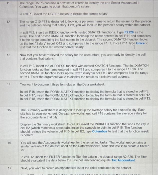
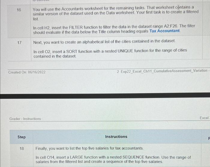
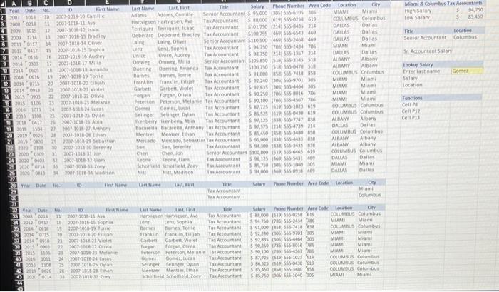
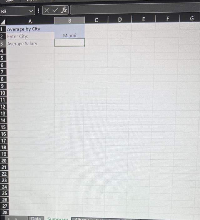
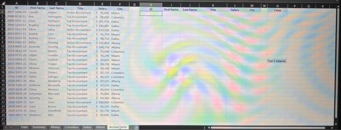
11 The range O5: P6 contains a new set of criteria to identify the one Senior Accountant in Columbus. You want to obtain that person's salary. In cell P8, insert the DGET function to extract the correct salary. 12. The range O10:P13 is designed to look up a person's name to return the salary for that person and the cell containing that salary. First, you will look up the person's salary within the dataset. In cell P12, insert an INDEX function with nested XMATCH functions. Type F2:126 as the array. The first nested XMATCH function looks up the name entered in cell P11 and compares it to the range containing the last names in the dataset. The second XMATCH function looks up the text "Salary" in cell 012 and compares it to the range F1:I1. In cell P11, type Unice to test that the function returns the correct salary. 13 Now that you have retrieved the salary for the accountant, you are ready to identify the cell that contains that salary. In cell P13, insert the ADDRESS function with nested XMATCH functions. The first XMATCH function looks up the name entered in cell P11 and compares it to the range F1 : F26. The second XMATCH function looks up the text "Salary" in cell 012 and compares it to the range A1:M1. Enter the arqument value to display the result as a relative cell address. 14 You want to document three formulas on the Data worksheet. In cell P16, insert the FORMULATEXT function to display the formula that is stored in cell P8. In cell P17, insert the FORMULATEXT function to display the formula that is stored in cell P12. In cell P18, insert the FORMULATEXT function to display the formula that is stored in cell P13. 15 The Summary worksheet is designed to look up the average salary for a specific city. Each city has its own worksheet. On each city worksheet, cell F 15 contains the average salary for the accountants in that city. Display the Summary worksheet. In cell B3, insert the INDIRECT function that uses the city in cell B2 (which matches a sheet tab). Insert the symbols to point to cell F15. The function should retrieve the value in cell F15. In cell B2, type Columbus to test that the function result is correct. 16 You will use the Accountants worksheet for the remaining tasks. That worksheet contains a similar version of the dataset used on the Data worksheet. Your first task is to create a filtered list. In cell H2; insert the FILTER function to filter the data in the dataset range A2: F26. The filter should evaluate if the data below the Title column heading equals Tax Accountant. 17 Next, you want to create an alphabetical list of the cities contained in the dataset. 16 You will use the Accountants worksheet for the remaining tasks. That worksheet ntains a similar version of the dataset used on the Data worksheet. Your first task is to create a filtered list. In cell H2, insert the FILTER function to filter the data in the dataset range A2:F26. The filter should evaluate if the data below the Title column heading equals Tax Accountant. 17 Next, you want to create an alphabetical list of the cities contained in the dataset. In cell O2, insert a SORT function with a nested UNIQUE function for the range of cities contained in the dataset. Created On: 06/16/2022 2. Exp22 Excel Ch11 CumulativeAssessment Variation. Grader - Instructions Step Instructions 18 Finally, you want to list the top five salaries for tax accountants. In cell O14, insert a LARGE function with a nested SEQUENCE function. Use the range of salaries from the filtered list and create a sequence of the top five salaries. B3 :fx A B C. D E F G 1 Average by City 2 Enter City: Miami Average Salary 11 The range O5: P6 contains a new set of criteria to identify the one Senior Accountant in Columbus. You want to obtain that person's salary. In cell P8, insert the DGET function to extract the correct salary. 12. The range O10:P13 is designed to look up a person's name to return the salary for that person and the cell containing that salary. First, you will look up the person's salary within the dataset. In cell P12, insert an INDEX function with nested XMATCH functions. Type F2:126 as the array. The first nested XMATCH function looks up the name entered in cell P11 and compares it to the range containing the last names in the dataset. The second XMATCH function looks up the text "Salary" in cell 012 and compares it to the range F1:I1. In cell P11, type Unice to test that the function returns the correct salary. 13 Now that you have retrieved the salary for the accountant, you are ready to identify the cell that contains that salary. In cell P13, insert the ADDRESS function with nested XMATCH functions. The first XMATCH function looks up the name entered in cell P11 and compares it to the range F1 : F26. The second XMATCH function looks up the text "Salary" in cell 012 and compares it to the range A1:M1. Enter the arqument value to display the result as a relative cell address. 14 You want to document three formulas on the Data worksheet. In cell P16, insert the FORMULATEXT function to display the formula that is stored in cell P8. In cell P17, insert the FORMULATEXT function to display the formula that is stored in cell P12. In cell P18, insert the FORMULATEXT function to display the formula that is stored in cell P13. 15 The Summary worksheet is designed to look up the average salary for a specific city. Each city has its own worksheet. On each city worksheet, cell F 15 contains the average salary for the accountants in that city. Display the Summary worksheet. In cell B3, insert the INDIRECT function that uses the city in cell B2 (which matches a sheet tab). Insert the symbols to point to cell F15. The function should retrieve the value in cell F15. In cell B2, type Columbus to test that the function result is correct. 16 You will use the Accountants worksheet for the remaining tasks. That worksheet contains a similar version of the dataset used on the Data worksheet. Your first task is to create a filtered list. In cell H2; insert the FILTER function to filter the data in the dataset range A2: F26. The filter should evaluate if the data below the Title column heading equals Tax Accountant. 17 Next, you want to create an alphabetical list of the cities contained in the dataset. 16 You will use the Accountants worksheet for the remaining tasks. That worksheet ntains a similar version of the dataset used on the Data worksheet. Your first task is to create a filtered list. In cell H2, insert the FILTER function to filter the data in the dataset range A2:F26. The filter should evaluate if the data below the Title column heading equals Tax Accountant. 17 Next, you want to create an alphabetical list of the cities contained in the dataset. In cell O2, insert a SORT function with a nested UNIQUE function for the range of cities contained in the dataset. Created On: 06/16/2022 2. Exp22 Excel Ch11 CumulativeAssessment Variation. Grader - Instructions Step Instructions 18 Finally, you want to list the top five salaries for tax accountants. In cell O14, insert a LARGE function with a nested SEQUENCE function. Use the range of salaries from the filtered list and create a sequence of the top five salaries. B3 :fx A B C. D E F G 1 Average by City 2 Enter City: Miami Average Salary