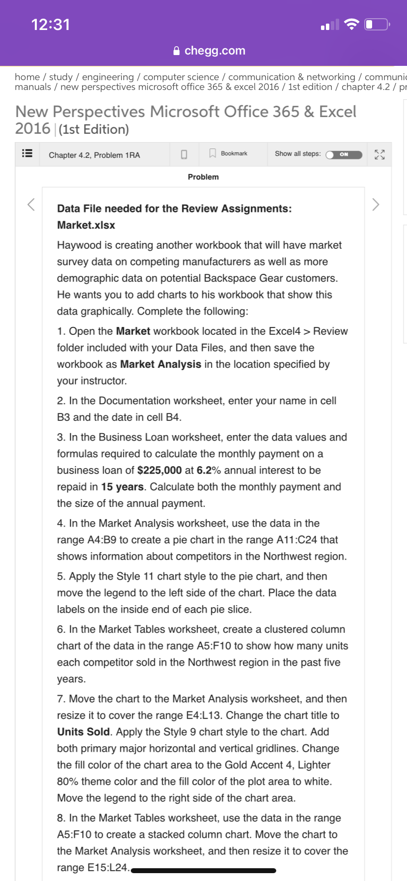
12:31 A chegg.com home / study / engineering / computer science / communication & networking / communi manuals / new perspectives microsoft office 365 & excel 2016 / 1st edition / chapter 4.2 / New Perspectives Microsoft Office 365 & Excel 2016 (1st Edition) IE Chapter 4.2, Problem 1RA 0 Bookmark Show all steps: ON Problem > Data File needed for the Review Assignments: Market.xlsx Haywood is creating another workbook that will have market survey data on competing manufacturers as well as more demographic data on potential Backspace Gear customers. He wants you to add charts to his workbook that show this data graphically. Complete the following: 1. Open the Market workbook located in the Excel4 > Review folder included with your Data Files, and then save the workbook as Market Analysis in the location specified by your instructor. 2. In the Documentation worksheet, enter your name in cell B3 and the date in cell B4. 3. In the Business Loan worksheet, enter the data values and formulas required to calculate the monthly payment on a business loan of $225,000 at 6.2% annual interest to be repaid in 15 years. Calculate both the monthly payment and the size of the annual payment. 4. In the Market Analysis worksheet, use the data in the range A4:B9 to create a pie chart in the range A11:C24 that shows information about competitors in the Northwest region. 5. Apply the Style 11 chart style to the pie chart, and then move the legend to the left side of the chart. Place the data labels on the inside end of each pie slice. 6. In the Market Tables worksheet, create a clustered column chart of the data in the range A5:F10 to show how many units each competitor sold in the Northwest region in the past five years. 7. Move the chart to the Market Analysis worksheet, and then resize it to cover the range E4:L13. Change the chart title to Units Sold. Apply the Style 9 chart style to the chart. Add both primary major horizontal and vertical gridlines. Change the fill color of the chart area to the Gold Accent 4, Lighter 80% theme color and the fill color of the plot area to white. Move the legend to the right side of the chart area. 8. In the Market Tables worksheet, use the data in the range A5:F10 to create a stacked column chart. Move the chart to the Market Analysis worksheet, and then resize it to cover the range E15:L24. 12:31 A chegg.com home / study / engineering / computer science / communication & networking / communi manuals / new perspectives microsoft office 365 & excel 2016 / 1st edition / chapter 4.2 / New Perspectives Microsoft Office 365 & Excel 2016 (1st Edition) IE Chapter 4.2, Problem 1RA 0 Bookmark Show all steps: ON Problem > Data File needed for the Review Assignments: Market.xlsx Haywood is creating another workbook that will have market survey data on competing manufacturers as well as more demographic data on potential Backspace Gear customers. He wants you to add charts to his workbook that show this data graphically. Complete the following: 1. Open the Market workbook located in the Excel4 > Review folder included with your Data Files, and then save the workbook as Market Analysis in the location specified by your instructor. 2. In the Documentation worksheet, enter your name in cell B3 and the date in cell B4. 3. In the Business Loan worksheet, enter the data values and formulas required to calculate the monthly payment on a business loan of $225,000 at 6.2% annual interest to be repaid in 15 years. Calculate both the monthly payment and the size of the annual payment. 4. In the Market Analysis worksheet, use the data in the range A4:B9 to create a pie chart in the range A11:C24 that shows information about competitors in the Northwest region. 5. Apply the Style 11 chart style to the pie chart, and then move the legend to the left side of the chart. Place the data labels on the inside end of each pie slice. 6. In the Market Tables worksheet, create a clustered column chart of the data in the range A5:F10 to show how many units each competitor sold in the Northwest region in the past five years. 7. Move the chart to the Market Analysis worksheet, and then resize it to cover the range E4:L13. Change the chart title to Units Sold. Apply the Style 9 chart style to the chart. Add both primary major horizontal and vertical gridlines. Change the fill color of the chart area to the Gold Accent 4, Lighter 80% theme color and the fill color of the plot area to white. Move the legend to the right side of the chart area. 8. In the Market Tables worksheet, use the data in the range A5:F10 to create a stacked column chart. Move the chart to the Market Analysis worksheet, and then resize it to cover the range E15:L24