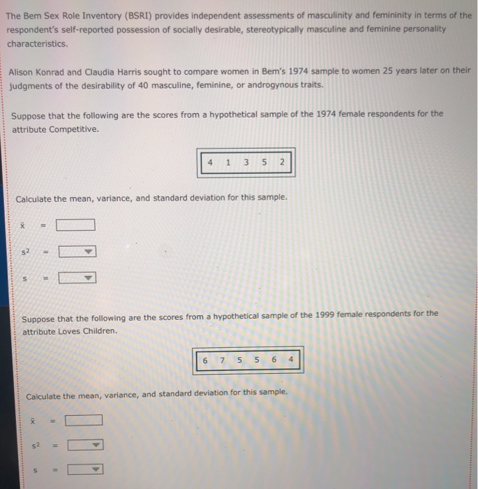
Question: 2. 3. 4. 5. 6. 7. The Bem Sex Role Inventory (BSRI) provides independent assessments of masculinity and femininity in terms of the respondent's self-reported
2.
3.
4.
5.
6.
7.
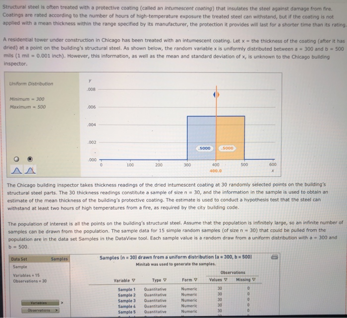
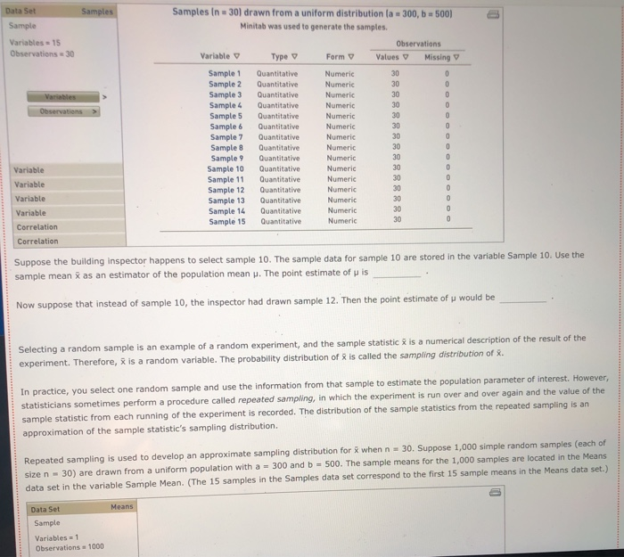
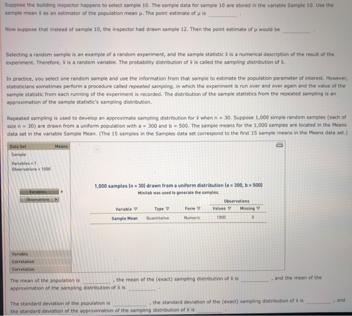
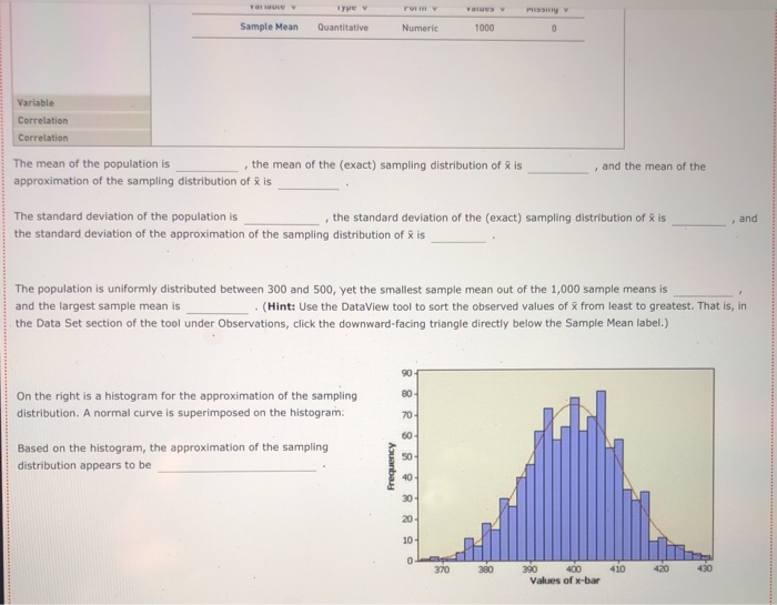
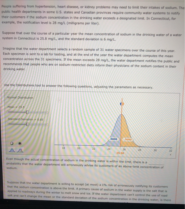
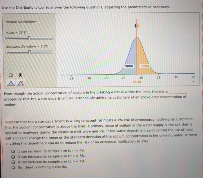
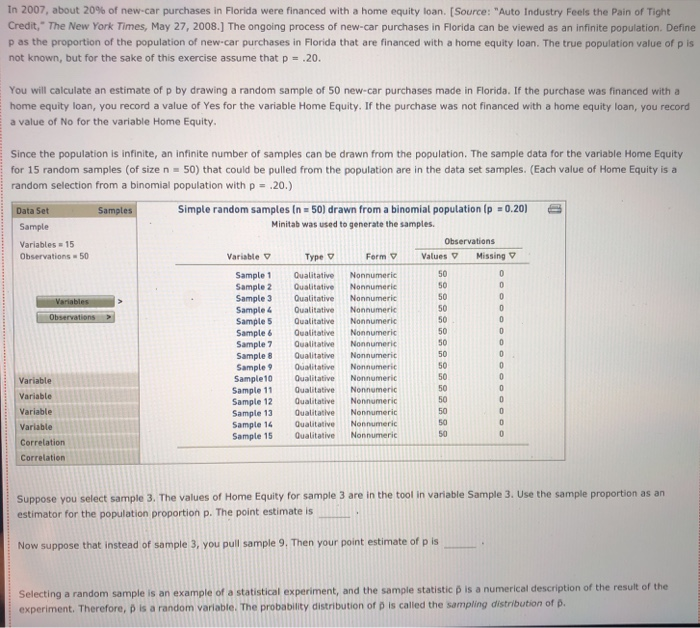
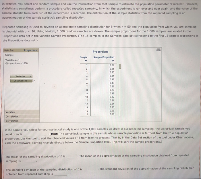
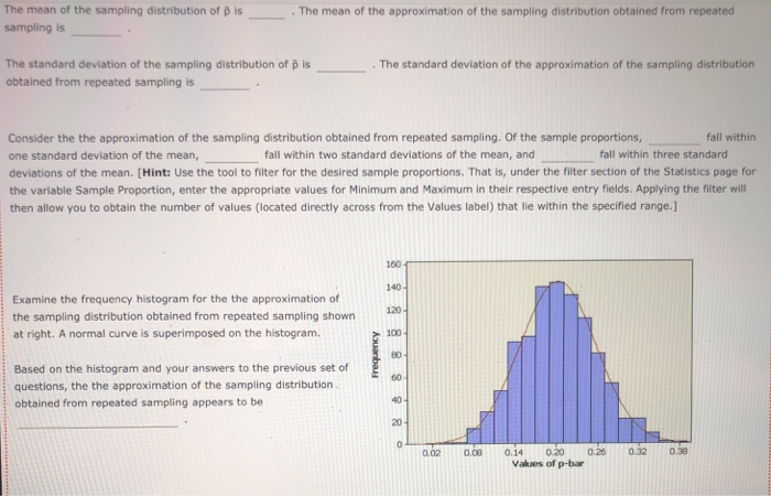
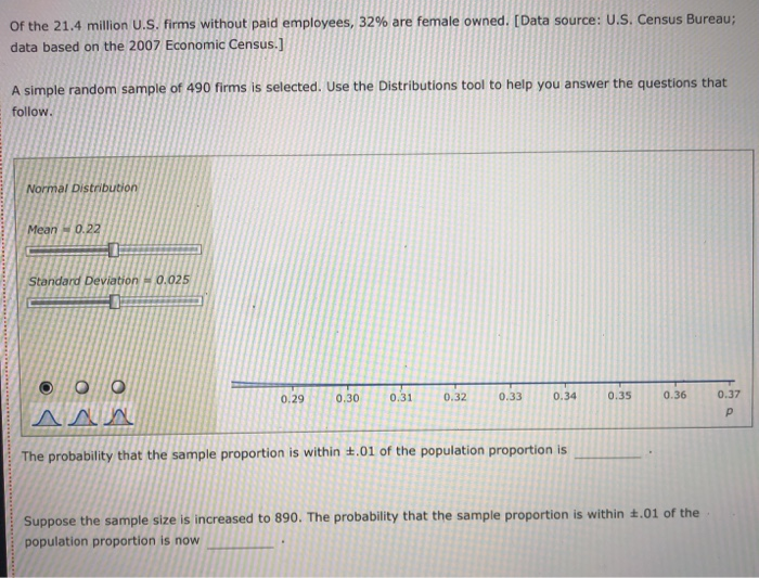
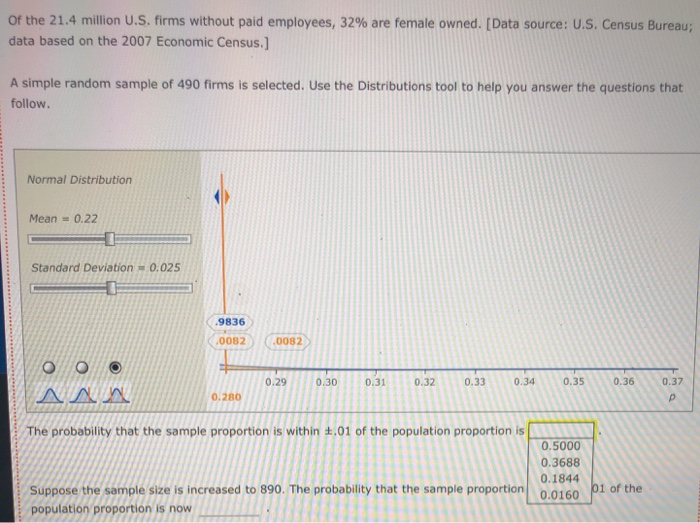
The Bem Sex Role Inventory (BSRI) provides independent assessments of masculinity and femininity in terms of the respondent's self-reported possession of socially desirable, stereotypically masculine and feminine personality characteristics. Alison Konrad and Claudia Harris sought to compare women in Bem's 1974 sample to women 25 years later on their judgments of the desirability of 40 masculine, feminine, or androgynous traits. Suppose that the following are the scores from a hypothetical sample of the 1974 female respondents for the attribute Competitive. 4 1 3 5 5 2 Calculate the mean, variance, and standard deviation for this sample. = s2 S Suppose that the following are the scores from a hypothetical sample of the 1999 female respondents for the attribute Loves Children. 6 7 5 5 6 4 Calculate the mean, variance, and standard deviation for this sample. X 52 $ Structural steel is often treated with a protective coating (called an intumescent coating) that insulates the steel against damage from fire. Coatings are rated according to the number of hours of high-temperature exposure the treated steel can withstand, but if the coating is not applied with a mean thickness within the range specified by its manufacturer, the protection it provides will last for a shorter time than its rating. A residential tower under construction in Chicago has been treated with an intumescent coating. Let the thickness of the coating (after it has dried) at a point on the building's structural steel. As shown below, the random variable x is uniformly distributed between a - 300 and b - 500 mils (1 mil = 0.001 inch). However, this information, as well as the mean and standard deviation of X, is unknown to the Chicago building inspector. y Uniform Distribution .008 Minimum - 300 Maximum = 500 .006 .004 .002 .5000 5000 .000 0 100 200 300 500 600 400 400.0 The Chicago building inspector takes thickness readings of the dried intumescent coating at 30 randomly selected points on the building's structural steel parts. The 30 thickness readings constitute a sample of size n = 30, and the information in the sample is used to obtain an estimate of the mean thickness of the building's protective coating. The estimate is used to conduct a hypothesis test that the steel can withstand at least two hours of high temperatures from a fire, as required by the city building code. The population of interest is all the points on the building's structural steel. Assume that the population is infinitely large, so an infinite number of samples can be drawn from the population. The sample data for 15 simple random samples (of size n = 30) that could be pulled from the population are in the data set Samples in the DataView tool. Each sample value is a random draw from a uniform distribution with a - 300 and b = 500 Samples Data Set Sample Variables - 15 Observations 30 Samples In - 30) drawn from a uniform distribution la : 300, b = 500) Minitab was used to generate the samples. Observations Variable y Type Form v Values Missing V Sample 1 Quantitative Numeric 30 0 Sample 2 Quantitative Numeric 30 Sample 3 Quantitative Numeric 30 Sample 4 Quantitative Numeric 30 Sample 5 Quantitative Numeric 30 0 0 Variables Observations O Samples Data Set Sample Variables 15 Observations = 30 Variables Observations Samples in 30) drawn from a uniform distribution la = 300, b = 500) Minitab was used to generate the samples. Observations Variable v Type 0 Form Values Missing Sample 1 Quantitative Numeric 30 0 Sample 2 Quantitative Numeric 30 0 Sample 3 Quantitative Numeric 30 0 Sample 4 Quantitative Numeric 30 0 Sample 5 Quantitative Numeric 30 0 Sample 6 Quantitative Numeric 30 0 Sample 7 Quantitative Numeric 30 0 Sample 8 Quantitative Numeric 30 0 Sample 9 Quantitative Numeric 30 0 Sample 10 Quantitative Numeric 30 0 Sample 11 Quantitative Numeric 30 0 Sample 12 Quantitative Numeric 30 0 Sample 13 Quantitative Numeric 30 0 Sample 14 Quantitative Numeric 30 0 Quantitative 30 Numeric Sample 15 0 Variable Variable Variable Variable Correlation Correlation Suppose the building Inspector happens to select sample 10. The sample data for sample 10 are stored in the variable Sample 10. Use the sample mean as an estimator of the population mean . The point estimate of pis Now suppose that instead of sample 10, the inspector had drawn sample 12. Then the point estimate of u would be Selecting a random sample is an example of a random experiment, and the sample statistic 3 is a numerical description of the result of the experiment. Therefore, & is a random variable. The probability distribution of is called the sampling distribution of . In practice, you select one random sample and use the information from that sample to estimate the population parameter of interest. However, statisticians sometimes perform a procedure called repeated sampling, in which the experiment is run over and over again and the value of the sample statistic from each running of the experiment is recorded. The distribution of the sample statistics from the repeated sampling is an approximation of the sample statistic's sampling distribution. Repeated sampling is used to develop an approximate sampling distribution for 8 when n = 30. Suppose 1,000 simple random samples (each of size n - 30) are drawn from a uniform population with a = 300 and b = 500. The sample means for the 1,000 samples are located in the Means data set in the variable Sample Mean. (The 15 samples in the Samples data set correspond to the first 15 sample means in the Means data set.) Means Data Set Sample Variables = 1 Observations = 1000 Suppose the building Inspector happens to select sample 10. The sample data for sample 10 are stored in the variable Sample 10. Use the sample mean as an estimator of the population mean p. The point estimate of u is Now suppose that instead of sample 10, the inspector had drawn sample 12. Then the point estimate of u would be Selecting a random sample is an example of a random experiment, and the sample statistic & is a numerical description of the result of the experiment. Therefore, & is a random variable. The probability distribution of R is called the sampling distribution of 8. In practice, you select one random sample and use the information from that sample to estimate the population parameter of interest. However, statisticians sometimes perform a procedure called repeated sampling, in which the experiment is run over and over again and the value of the sample statistic from each running of the experiment is recorded. The distribution of the sample statistics from the repeated sampling is an approximation of the sample statistic's sampling distribution. Repeated sampling is used to develop an approximate sampling distribution for 8 when n = 30. Suppose 1,000 simple random samples (each of size n - 30) are drawn from a uniform population with a - 300 and b - 500. The sample means for the 1,000 samples are located in the Means data set in the variable Sample Mean. (The 15 samples in the Samples data set correspond to the first 15 sample means in the Means data set.) Data Set Means Sample Variables 1 Observations 1000 Variables Observations 1,000 samples in = 30) drawn from a uniform distribution la = 300, b = 500) Minitab was used to generate the samples. Observations Variable v Type V Form v Values v Missing Sample Mean Quantitative Numeric 1000 0 Variable Correlation Correlation . and the mean of the The mean of the population is the mean of the (exact) sampling distribution of is approximation of the sampling distribution of is and The standard deviation of the population is the standard deviation of the (exact) sampling distribution of is the standard deviation of the approximation of the sampling distribution of X is TE Type r Yates Sample Mean Quantitative Numeric 1000 0 Variable Correlation Correlation The mean of the population is the mean of the (exact) sampling distribution of X is approximation of the sampling distribution of X is and the mean of the and The standard deviation of the population is the standard deviation of the (exact) sampling distribution of X is the standard deviation of the approximation of the sampling distribution of Ris The population is uniformly distributed between 300 and 500, yet the smallest sample mean out of the 1,000 sample means is and the largest sample mean is . (Hint: Use the DataView tool to sort the observed values of from least to greatest. That is, in the Data Set section of the tool under Observations, click the downward-facing triangle directly below the Sample Mean label.) 90 80- On the right is a histogram for the approximation of the sampling distribution. A normal curve is superimposed on the histogram. 70 60 Based on the histogram, the approximation of the sampling distribution appears to be 50 Frequency 40 30 20 10 0 370 390 410 390 400 Values of x-bar People suffering from hypertension, heart disease, or kidney problems may need to limit their intakes of sodium. The public health departments in some U.S. states and Canadian provinces require community water systems to notify their customers if the sodium concentration in the drinking water exceeds a designated limit. In Connecticut, for example, the notification level is 28 mg/L (milligrams per liter). Suppose that over the course of a particular year the mean concentration of sodium in the drinking water of a water system in Connecticut is 25.8 mg/L, and the standard deviation is 6 mg/L. Imagine that the water department selects a random sample of 31 water specimens over the course of this year. Each specimen is sent to a lab for testing, and at the end of the year the water department computes the mean concentration across the 31 specimens. If the mean exceeds 28 mg/L, the water department notifies the public and recommends that people who are on sodium-restricted diets inform their physicians of the sodium content in their drinking water. Use the Distributions tool to answer the following questions, adjusting the parameters as necessary. Normal Distribution Mean = 25.5 Standard Deviation = 0.85 .5000 .5000 18 20 22 24 28 30 26 25.50 32 Even though the actual concentration of sodium in the drinking water is within the limit, there is a probability that the water department will erroneously advise its customers of an above-limit concentration of sodium Suppose that the water department is willing to accept (at most) a 1% risk of erroneously notifying its customers that the sodium concentration is above the limit. A primary cause of sodium in the water supply is the salt that is applied to roadways during the winter to melt snow and ice. If the water department can't control the use of road salt and can't change the mean or the standard deviation of the sodium concentration in the drinking water, is there Use the Distributions tool to answer the following questions, adjusting the parameters as necessary. Normal Distribution Mean = 25.5 Standard Deviation = 0.85 .5000 .5000 20 18 22 24 28 30 32 26 25.50 X Even though the actual concentration of sodium in the drinking water is within the limit, there is a probability that the water department will erroneously advise its customers of an above-limit concentration of sodium Suppose that the water department is willing to accept (at most) a 1% risk of erroneously notifying its customers that the sodium concentration is above the limit. A primary cause of sodium in the water supply is the salt that is applied to roadways during the winter to melt snow and ice. If the water department can't control the use of road salt and can't change the mean or the standard deviation of the sodium concentration in the drinking water, is there anything the department can do to reduce the risk of an erroneous notification to 1%? It can increase its sample size to n - 48. It can increase its sample size to n = 88. O It can increase its sample size to n - 40. No, there is nothing it can do. In 2007, about 20% of new-car purchases in Florida were financed with a home equity loan. (Source: "Auto Industry Feels the pain of Tight Credit," The New York Times, May 27, 2008.] The ongoing process of new-car purchases in Florida can be viewed as an infinite population. Define p as the proportion of the population of new-car purchases in Florida that are financed with a home equity loan. The true population value of pis not known, but for the sake of this exercise assume that p = .20. You will calculate an estimate of p by drawing a random sample of 50 new-car purchases made in Florida. If the purchase was financed with a home equity loan, you record a value of Yes for the variable Home Equity. If the purchase was not financed with a home equity loan, you record a value of No for the variable Home Equity. 0 0 Since the population is infinite, an infinite number of samples can be drawn from the population. The sample data for the variable Home Equity for 15 random samples of size n = 50) that could be pulled from the population are in the data set samples. (Each value of Home Equity is a random selection from a binomial population with p = .20.) Data Set Samples Simple random samples in = 50) drawn from a binomial population (p = 0.20) Sample Minitab was used to generate the samples. Variables 15 Observations Observations - 50 Variable Type 0 Form Values Missing Sample 1 Qualitative Nonnumeric 50 Sample 2 Qualitative Nonnumeric 50 Variables Sample 3 Qualitative Nonnumeric 50 Sample 4 Qualitative Nonnumeric 50 Observations Sample 5 Qualitative Nonnumeric 50 Sample 6 Qualitative Nonnumeric 50 Sample 7 Qualitative Nonnumeric 50 0 Sample 8 Qualitative Nonnumeric 50 Sample 9 Qualitative Nonnumeric 50 Variable Sample 10 Qualitative Nonnumeric 50 Sample 11 Variable Qualitative Nonnumeric 50 Sample 12 Qualitative Nonnumeric Variable Sample 13 Qualitative Nonnumeric 50 Variable Sample 14 Qualitative Nonnumeric 50 0 Sample 15 Correlation Qualitative Nonnumeric Correlation 0 0 0 0 0 0 0 O 50 0 0 50 0 Suppose you select sample 3. The values of Home Equity for sample 3 are in the tool in variable Sample 3. Use the sample proportion as an estimator for the population proportion p. The point estimate is Now suppose that instead of sample 3, you pull sample 9. Then your point estimate of pis Selecting a random sample is an example of a statistical experiment, and the sample statistic p is a numerical description of the result of the experiment. Therefore, D is a random variable. The probability distribution of p is called the sampling distribution of p. In practice, you select one random sample and use the information from that sample to estimate the population parameter of interest. However, statisticians sometimes perform a procedure called repeated sampling, in which the experiment is run over and over again, and the value of the sample statistic from each run of the experiment is recorded. The distribution of the sample statistics from the repeated sampling is an approximation of the sample statistic's sampling distribution. Repeated sampling is used to develop an approximate sampling distribution for p when n = 50 and the population from which you are sampling is binomial with p - 20. Using Minitab, 1,000 random samples are drawn. The sample proportions for the 1,000 samples are located in the Proportions data set in the variable Sample Proportion. (The 15 samples in the Samples data set correspond to the first 15 sample proportions in the Proportions data set.) Data Set Proportions Sample Variables = 1 Observations - 1000 Proportions Sample Proportion V Sample V 1 2 3 4 Variables Observations 5 6 7 8 0.24 0.26 0.20 0.34 0.18 0.18 0.26 0.20 0.12 0.32 0.26 0.24 0.20 0.28 0.20 9 10 11 12 13 14 15 Variable Correlation Correlation If the sample you select for your statistical study is one of the 1,000 samples we drew in our repeated sampling, the worst-luck sample you could draw is (Hint: The worst-luck sample is the sample whose sample proportion is farthest from the true population proportion. Use the tool to sort the observed values of p from least to greatest. That is, in the Data Set section of the tool under Observations, click the downward pointing triangle directly below the Sample Proportion label. This will sort the sample proportions.) The mean of the approximation of the sampling distribution obtained from repeated The mean of the sampling distribution of Dis sampling is . The standard deviation of the approximation of the sampling distribution The standard deviation of the sampling distribution of Dis obtained from repeated sampling is The mean of the sampling distribution of Dis sampling is . The mean of the approximation of the sampling distribution obtained from repeated The standard deviation of the sampling distribution of pis obtained from repeated sampling is The standard deviation of the approximation of the sampling distribution Consider the the approximation of the sampling distribution obtained from repeated sampling. Of the sample proportions, fall within one standard deviation of the mean, fall within two standard deviations of the mean, and fall within three standard deviations of the mean. (Hint: Use the tool to filter for the desired sample proportions. That is, under the filter section of the Statistics page for the variable Sample Proportion, enter the appropriate values for Minimum and Maximum in their respective entry fields. Applying the filter will then allow you to obtain the number of values (located directly across from the Values label) that lie within the specified range.] 160 140 120- Examine the frequency histogram for the the approximation of the sampling distribution obtained from repeated sampling shown at right. A normal curve is superimposed on the histogram. 100 Frequency 80 60 Based on the histogram and your answers to the previous set of questions, the the approximation of the sampling distribution obtained from repeated sampling appears to be 40 20 0 0.02 0.08 0.32 0.38 0.14 0.20 0.26 Values of p-bar Of the 21.4 million U.S. firms without paid employees, 32% are female owned. [Data source: U.S. Census Bureau; data based on the 2007 Economic Census.] A simple random sample of 490 firms is selected. Use the Distributions tool to help you answer the questions that follow. Normal Distribution Mean -0.22 Standard Deviation 0.025 0.29 0.30 0.31 0.32 0.33 0.34 0.35 0.36 0.37 The probability that the sample proportion is within 4.01 of the population proportion is Suppose the sample size is increased to 890. The probability that the sample proportion is within 1.01 of the population proportion is now of the 21.4 million U.S. firms without paid employees, 32% are female owned. [Data source: U.S. Census Bureau; data based on the 2007 Economic Census.] A simple random sample of 490 firms is selected. Use the Distributions tool to help you answer the questions that follow. Normal Distribution Mean = 0.22 Standard Deviation = 0.025 D 19836 0082 0082 AA 0.29 0.30 0.31 0.32 0.33 0.34 0.35 0.36 0.37 P 0.280 The probability that the sample proportion is within 4.01 of the population proportion is 0.5000 0.3688 0.1844 0.0160 01 of the Suppose the sample size is increased to 890. The probability that the sample proportion population proportion is now You are interested in estimating the mean of a population. You plan to take a random sample from the population and use the sample's mean as an estimate of the population mean. Assuming that the population from which you select your sample is normal, which of the statements about are true? Check all that apply. It follows a normal distribution only for sufficiently large sample sizes. Its expected value is equal to the value of the population mean. It follows a uniform distribution only for large sample sizes. The variance of its sampling distribution is equal to the sample variance divided by the sample size. It follows a normal distribution for any sample size. When the population is infinite, the standard deviation of its sampling distribution is equal to the standard deviation of the population divided by the square root of the sample size. DI Assume that the population from which you select your sample is not normal. Which of the statements about & are true? Check all that apply. It follows a normal distribution for any sample size. Its expected value is equal to the value of the population mean. The variance of its sampling distribution is equal to the sample variance divided by the sample size. When the population is infinite, the standard deviation of its sampling distribution is equal to the standard deviation of the population divided by the square root of the sample size. It follows a normal distribution only for sufficiently large sample sizes