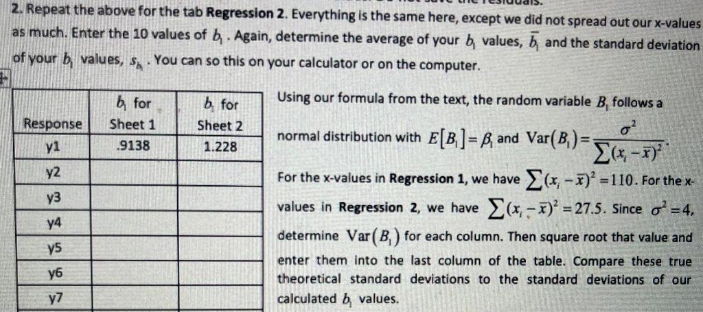
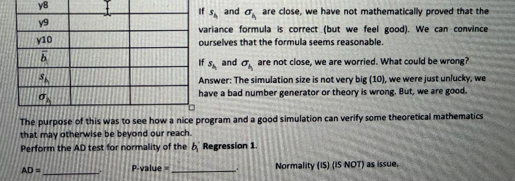
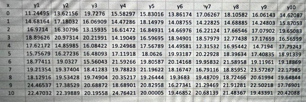
2. Repeat the above for the tab Regression 2. Everything is the same here, except we did not spread out our x-values as much. Enter the 10 values of b. Again, determine the average of your b, values, 5, and the standard deviation of your b, values, sy. You can so this on your calculator or on the computer. Using our formula from the text, the random variable B. follows a Response yi b for Sheet 1 .9138 b for Sheet 2 1.228 y2 y3 normal distribution with E[B]= B and Var(B)=; 2(4,-1) For the x-values in Regression 1, we have (x, - 7) =110. For the x- values in Regression 2, we have (x, - 7)' = 27.5. Since o =4. determine Var(B) for each column. Then square root that value and enter them into the last column of the table. Compare these true theoretical standard deviations to the standard deviations of our calculated b values. y4 y5 y7 y8 y9 if s, and on are close, we have not mathematically proved that the variance formula is correct (but we feel good). We can convince ourselves that the formula seems reasonable. y10 b and on $ If Sa are not close, we are worried. What could be wrong? Answer: The simulation size is not very big (10), we were just unlucky, we have a bad number generator or theory is wrong. But, we are good. 0 The purpose of this was to see how a nice program and a good simulation can verify some theoretical mathematics that may otherwise be beyond our reach. Perform the AD test for normality of the b Regression 1. AD = P-value = Normality (IS) (IS NOT) as issue. yio *O Nm 00 4 y1 y2 y3 y4 y5 y6 y7 y8 y9 11.24495 13.62156 19.7276 15.58297 15.83016 13.86174 17.06267 18.10582 16.06143 14.62087 14.68164 17.18032 16.06909 14.47286 18.14979 14.08755 14.22825 14.68885 14.24803 15.87053 16.9714 16.30796 13.15935 16.61472 16.84931 14.66976 16.22124 17.66546 17.07902 19.65083 18.89626 20.97314 20.21991 14.19049 16.59695 18.94901 18.57979 12.77438 17.17659 16.56599 17.62172 14.85985 16.08422 19.24968 17.56789 14.49581 12.31532 16.95442 14.7194 17.79243 15.75679 16.27236 16.48093 17.11918 18.0626 19.93187 20.22928 18.39634 17.40835 18.91339 18.77411 19.0327 15.56043 21.59266 19.80587 20.14168 19.95832 21.58958 19.11961 19.18869 19.21354 19.37404 18.41283 19.78823 21.19622 18.16747 16.79116 18.85952 23.57267 22.17985 18.12916 19.53428 19.74904 20.35217 19.26444 19.3683 19.48709 18.72466 20.61994 19.64844 24.46537 17.38529 20.68872 18.68901 20.82958 16.27341 21.29469 21.91281 22.50218 17.76901 22.47032 22.39889 20.19558 24.76421 20.00005 19.46852 20.68139 21.48367 19.43391 20.42088 5 9 10 2. Repeat the above for the tab Regression 2. Everything is the same here, except we did not spread out our x-values as much. Enter the 10 values of b. Again, determine the average of your b, values, 5, and the standard deviation of your b, values, sy. You can so this on your calculator or on the computer. Using our formula from the text, the random variable B. follows a Response yi b for Sheet 1 .9138 b for Sheet 2 1.228 y2 y3 normal distribution with E[B]= B and Var(B)=; 2(4,-1) For the x-values in Regression 1, we have (x, - 7) =110. For the x- values in Regression 2, we have (x, - 7)' = 27.5. Since o =4. determine Var(B) for each column. Then square root that value and enter them into the last column of the table. Compare these true theoretical standard deviations to the standard deviations of our calculated b values. y4 y5 y7 y8 y9 if s, and on are close, we have not mathematically proved that the variance formula is correct (but we feel good). We can convince ourselves that the formula seems reasonable. y10 b and on $ If Sa are not close, we are worried. What could be wrong? Answer: The simulation size is not very big (10), we were just unlucky, we have a bad number generator or theory is wrong. But, we are good. 0 The purpose of this was to see how a nice program and a good simulation can verify some theoretical mathematics that may otherwise be beyond our reach. Perform the AD test for normality of the b Regression 1. AD = P-value = Normality (IS) (IS NOT) as issue. yio *O Nm 00 4 y1 y2 y3 y4 y5 y6 y7 y8 y9 11.24495 13.62156 19.7276 15.58297 15.83016 13.86174 17.06267 18.10582 16.06143 14.62087 14.68164 17.18032 16.06909 14.47286 18.14979 14.08755 14.22825 14.68885 14.24803 15.87053 16.9714 16.30796 13.15935 16.61472 16.84931 14.66976 16.22124 17.66546 17.07902 19.65083 18.89626 20.97314 20.21991 14.19049 16.59695 18.94901 18.57979 12.77438 17.17659 16.56599 17.62172 14.85985 16.08422 19.24968 17.56789 14.49581 12.31532 16.95442 14.7194 17.79243 15.75679 16.27236 16.48093 17.11918 18.0626 19.93187 20.22928 18.39634 17.40835 18.91339 18.77411 19.0327 15.56043 21.59266 19.80587 20.14168 19.95832 21.58958 19.11961 19.18869 19.21354 19.37404 18.41283 19.78823 21.19622 18.16747 16.79116 18.85952 23.57267 22.17985 18.12916 19.53428 19.74904 20.35217 19.26444 19.3683 19.48709 18.72466 20.61994 19.64844 24.46537 17.38529 20.68872 18.68901 20.82958 16.27341 21.29469 21.91281 22.50218 17.76901 22.47032 22.39889 20.19558 24.76421 20.00005 19.46852 20.68139 21.48367 19.43391 20.42088 5 9 10