

Question: 3 . 1 . 1 . 1 CONVERTING DISTRIBUTED LOADS TO POINT LOADS Unfortunately, both our live and dead loads are distributed loads. We have
CONVERTING DISTRIBUTED LOADS TO POINT LOADS
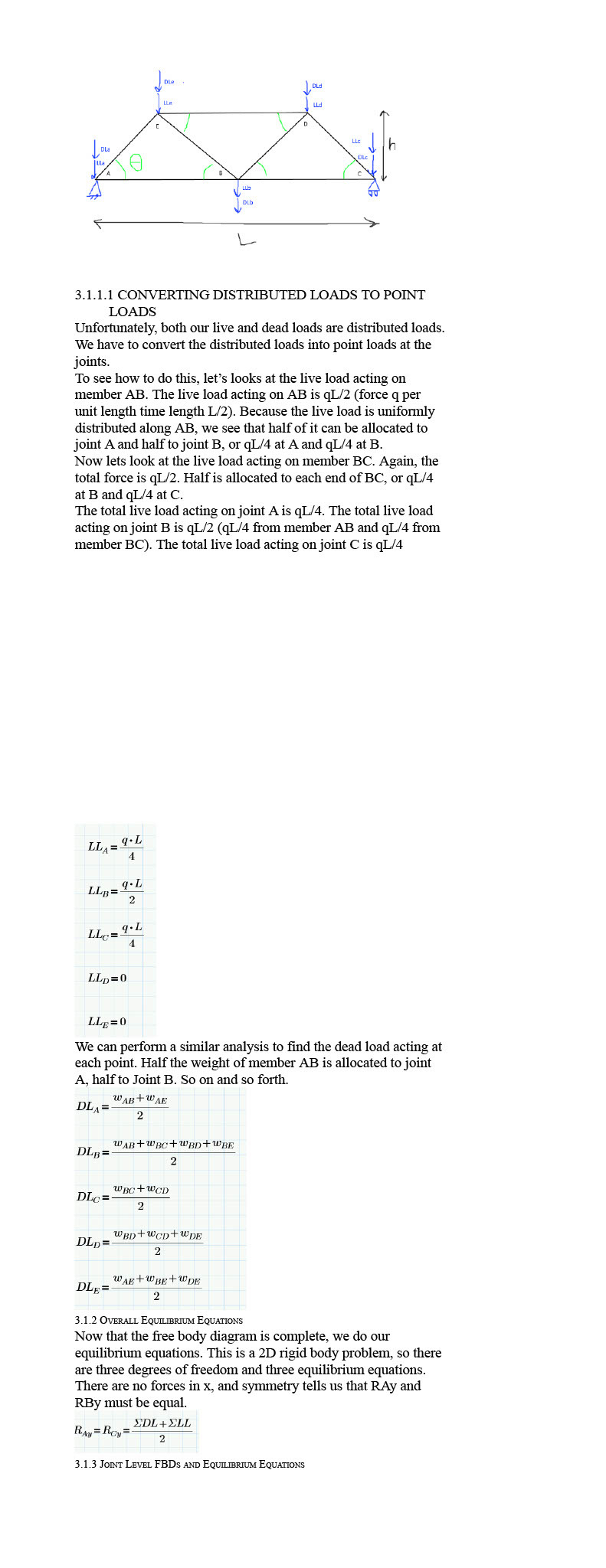
Unfortunately, both our live and dead loads are distributed loads. We have to convert the distributed loads into point loads at the joints.
To see how to do this, let's looks at the live load acting on member AB The live load acting on AB is force per unit length time length Because the live load is uniformly distributed along AB we see that half of it can be allocated to joint A and half to joint or at A and at B
Now lets look at the live load acting on member BC Again, the total force is Half is allocated to each end of BC or qL at and at C
The total live load acting on joint A is The total live load acting on joint B is from member AB and from member BC The total live load acting on joint C is
We can perform a similar analysis to find the dead load acting at each point. Half the weight of member is allocated to joint A half to Joint B So on and so forth.
Overall Equilibrium Equations
Now that the free body diagram is complete, we do our equilibrium equations. This is a D rigid body problem, so there are three degrees of freedom and three equilibrium equations. There are no forces in x and symmetry tells us that RAy and RBy must be equal.
Jont Level FBDs and Equilibrium Equations CONVERTING DISTRIBUTED LOADS TO POINT LOADS
Unfortunately, both our live and dead loads are distributed loads. We have to convert the distributed loads into point loads at the joints.
To see how to do this, let's looks at the live load acting on member AB The live load acting on AB is force per unit length time length Because the live load is uniformly distributed along AB we see that half of it can be allocated to joint A and half to joint or at A and at B
Now lets look at the live load acting on member BC Again, the total force is Half is allocated to each end of BC or qL at and at C
The total live load acting on joint A is The total live load acting on joint B is from member AB and from member BC The total live load acting on joint C is
We can perform a similar analysis to find the dead load acting at each point. Half the weight of member is allocated to joint A half to Joint B So on and so forth.
Overall Equilibrium Equations
Now that the free body diagram is complete, we do our equilibrium equations. This is a D rigid body problem, so there are three degrees of freedom and three equilibrium equations. There are no forces in x and symmetry tells us that RAy and RBy must be equal.
Jont Level FBDs and Equilibrium Equations
Step by Step Solution
There are 3 Steps involved in it
1 Expert Approved Answer
Step: 1 Unlock

Question Has Been Solved by an Expert!
Get step-by-step solutions from verified subject matter experts
Step: 2 Unlock
Step: 3 Unlock