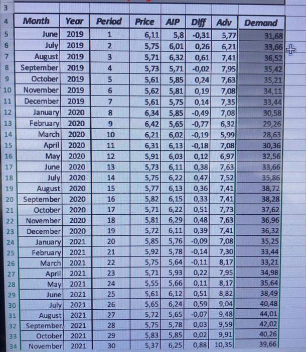
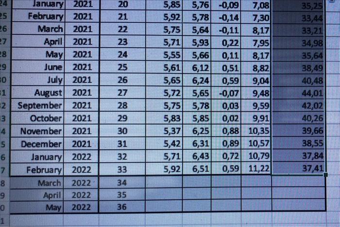
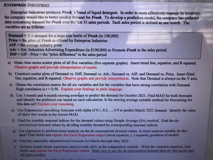
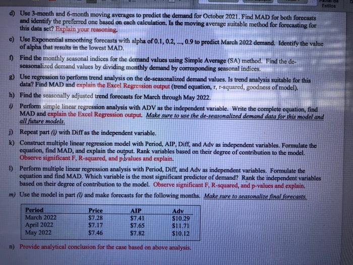
Question: 3 4 Demand 31,68 5 5 6 7 33,66 + 8 9 10 11 12 13 14 15 16 17 18 Month Year June 2019

3 4 Demand 31,68 5 5 6 7 33,66 + 8 9 10 11 12 13 14 15 16 17 18 Month Year June 2019 July 2019 August 2019 September 2019 October 2019 November 2019 December 2019 January 2020 February 2020 March 2020 April 2020 May 2020 June 2020 July 2020 August 2020 September 2020 October 2020 November 2020 December 2020 January 2021 February 2021 March 2021 April 2021 May 2021 June 2021 July 2021 August 2021 September 2021 October 2021 November 2021 Perlod 1 2 3 4 5 6 7 8 9 10 11 12 13 14 15 16 17 18 19 20 21 22 23 24 25 26 27 28 29 30 Price AIP Diff Ady 6,11 5,8 -0,31 5,77 5,75 6,01 0,26 6,21 5,71 6,32 0,61 7,41 5,73 5,71 -0,02 7,95 5,61 5,85 0,24 7,63 5,62 5,81 0,19 7,08 5,61 5,75 0,14 7,35 6,34 5,85 -0,49 7,08 6,42 5,65 -0,77 6,32 6,216,02 -0,19 5,99 6,31 6,13 -0,18 7,08 5,91 6,03 0,12 6,97 5,73 6,11 0,38 7,63 5,75 6,22 0,47 7,52 5,77 6,13 0,36 7,41 5,82 6,15 0,33 7,41 5,71 6,22 0,51 7,73 5,81 6,29 0,48 7,63 5,72 6,11 0,39 7,41 5,85 5,76 -0,09 7,08 5,92 5,78 -0,14 7,30 5,75 5,64 -0,11 8,17 5,71 5,93 0,22 7,95 5,55 5,66 0,11 8,17 5,61 6,12 0,51 8,82 5,656,24 0,59 9,04 5,72 5,65 -0,07 9,48 5,75 5,78 0,03 9,59 5,83 5,85 0,02 9,91 5,371 6,25 0,88 10,35 19 20 36,52 35,42 35,21 34,11 33,44 30,58 29,26 28,63 30,36 32,56 33,66 35,86 38,72 38,28 37,62 36,96 36,32 35,25 33,44 33,21 34,98 35,64 38,49 40,48 44,01 42,02 40,26 39,66 21 22 23 NN NN 24 25 26 27 28 29 30 31 32 2 www 33 m 34 1 24 25 26 27 28 20 21 22 COahin 23 24 25 19 30 1 2 13 14 January 2021 February 2021 March 2021 April 2021 May 2021 June 2021 July 2021 August 2021 September 2021 October 2021 November 2021 December 2021 January 2022 February 2022 March 2022 April 2022 May 2022 -0,07 5,85 5,76 -0,09 7,08 5,92 5,78 -0,14 7,30 5,75 5,64 -0,11 8,17 5,71 5,93 0,22 7,95 5,55 5,66 0,11 8,17 5,61 6,12 0,51 8,82 5,65 6,24 0,59 9,04 5,725,65 9,48 5,75 5,78 0,03 9,59 5,83 5,85 0,02 9,91 5,37 6,25 0,88 10,35 5,42 6,31 0,89 10,57 5,71 6,43 0,72 10,79 5,92 6,51 0,59 11,22 26 27 28 29 30 31 32 33 35,25 33,44 33,21 34,98 35,64 38,49 40,48 44,01 42,02 40,26 39,66 38,55 37,84 37,41 5 6 7 8 34 DOO 9 0 1 35 36 ENTERPRISE INDUSTRIES Enterprise Industries produces Fresh, a brand of liquid detergent. In order to more effectively manage its inventory, the company would like to better predict demand for Fresh. To develop a prediction model, the company has gathered data concerning demand for Fresh over the last 33 sales periods. Each sales period is defined as one month. The variables are as follows: Demand-Y-demand for a large size bottle of Fresh (in 100,000) Price = the price of Fresh as offered by Enterprise Industries AIP the average industry price Ady - Ent. Industries Advertising Expenditure (in $100,000) to Promote Fresh in the sales period. Diff -- AIP - Price = the "price difference in the sales period a) Make time series scatter plots of all five variables (five separate graphs). Insert trend line, equation, and R-squared Observe graphs and provide interpretation of results. b) Construct scatter plots of Demand vs. Diff, Demand vs. Adv, Demand vs. AIP, and Demand vs. Price. Insert fitted line, equation, and R-squared. Observe graphs and provide interpretation. Note that Demand is always on the Y axis. c) Obtain the correlation matrix for all six variables and list the variables that have strong correlation with Demand. High correlation is r >0.50. Explain your findings in plain language. dy Use 3-month and 6-month moving averages to predict the demand for October 2021. Find MAD for both forecasts and identify the preferred one based on each calculation. Is the moving average suitable method for forecasting for this data set? Explain your reasoning. c) Use Exponential smoothing forecasts with alpha of 0.1, 0.2, 0.9 to predict March 2022 demand. Identify the value of alpha that results in the lowest MAD. f) Find the monthly seasonal indices for the demand values using Simple Average (SA) method. Find the de- seasonalized demand values by dividing monthly demand by corresponding seasonal indices. g) Use regression to perform trend analysis on the de-seasonalized demand values. Is trend analysis suitable for this data? Find MAD and explain the Excel Regression output (trend equation, r, 1-squared, goodness of model) h) Find the seasonally adjusted trend forecasts for March through May 2022 0 Perform simple linear regression analysis with ADV as the independent variable. Write the complete equation, find MAD and explain the Excel Regression output. Make sure to use the de-seasonalized demand data for this model and all future models. Estilos d) Use 3-month and 6-month moving averages to predict the demand for October 2021. Find MAD for both forecasts and identify the preferred one based on cach calculation. Is the moving average suitable method for forecasting for this data set? Explain your reasoning, e) Use Exponential smoothing forecasts with alpha of 0.1, 0.2, ..., 0.9 to predict March 2022 demand. Identify the value of alpha that results in the lowest MAD. 1) Find the monthly scasonal indices for the demand values using Simple Average (SA) method. Find the de- seasonalized demand values by dividing monthly demand by corresponding seasonal indices, g) Use regression to perform trend analysis on the de-seasonalized demand values. Is trend analysis suitable for this data? Find MAD and explain the Excel Regression output (trend equation, r, r-squared, goodness of model). h) Find the seasonally adjusted trend forecasts for March through May 2022. Perform simple linear regression analysis with ADV as the independent variable. Write the complete equation, find MAD and explain the Excel Regression output. Make sure to use the de-seasonalized demand data for this model an all future models j) Repeat part (0 with Diff as the independent variable. k) Construct multiple linear regression model with Period, AIP, Diff, and Adv as independent variables. Formulate the equation, find MAD, and explain the output. Rank variables based on their degree of contribution to the model. Observe significant F, R-squared, and p-values and explain. D Perform multiple linear regression analysis with Period, Diff, and Ady as independent variables. Formulate the equation and find MAD. Which variable is the most significant predictor of demand? Rank the independent variables based on their degree of contribution to the model. Observe significant F, R-squared, and p-values and explain. m) Use the model in part (1) and make forecasts for the following months. Make sure to seasonalize final forecasts. Period March 2022 April 2022 May 2022 Price S7.28 S7.17 $7.46 AIP $7.41 $7.65 $7.82 Ady SI0.29 SILI S10.12 n) Provide analytical conclusion for the case based on above analysis

Step by Step Solution

There are 3 Steps involved in it

1 Expert Approved Answer

Step: 1 Unlock blur-text-image

Question Has Been Solved by an Expert!

Get step-by-step solutions from verified subject matter experts

Step: 2 Unlock

Step: 3 Unlock

Students Have Also Explored These Related General Management Questions!

The flow of manufacturing costs through the ledger accounts of Superior Locks, Inc., in the current year is illustrated below in summarized form. Instructions Indicate the amounts requested below....

Question 2 of 8 This question: 1 point(s) possible Aggressive versus conservative seasonal funding strategy Dynabase Tool has forecast its total funding requirements for the coming year as shown in...

Forecast the Demand ans calculate the overall forecast error measures (MAD, MSE, MAPE) in the following table using 4-month moving approach. B D E G H - K M o F 1 Forecast the demand and calculate...

B H Present Value of Annuity $1.00 in Arrears 1 2 3 Interest Periods Interest Periods 4 5 6 7 7 8 8 9 10 11 12 13 14 15 16 17 18 19 20 21 22 23 24 25 26 Rate 2.0% 2.5% 3.0% 3.5% 4.0% 4.5% 5.0% 5.5%...

C11 30200 A B D E N- 3 1) Prepare the Income Statement, Balance Sheet and Statement of Cash Flows for YoyoDyne 4. Propulsion Systems (YPS) using the following information. 2) Include Common Size...

I NEED HELP CALCULATING RATIOS AND CASH FLOWS. PLEASE SHOW HOW TO SOLVE USING EXCEL FOR EXAMPLE: =SUM(B4:B10)-B15 DATA: NEED CASH FLOWS NEED RATIOS C11 30200 A B D E N- 3 1) Prepare the Income...

Jan.3 Sell merchandise on account to M. Knast $5,100, invoice no. 825, and to C. Ryder $1,900, invoice no. 826. 5 Purchase merchandise from R. Drifter $5,000 and N. Sova $2,200, terms n/30. 7 Receive...

1 Nunya Business started operations on july 1, 2019 with an initial issuance of common stock. $31,700 2 Nunya business performed services for one month on account. $26000 3. Nunya Business has...

Please help me with this solution This is intended to get you to think about different graphical tools to describe data that is collected. It is your job to interpret what you see in the data and...

Imagine that it is January 2021, and you have just accepted the chief financial officer (CFO) position at Hays County Integrated Delivery System (IDS), hereafter referred to as County. You will be...

Explain why the renewability feature makes term insurance more attractive to some buyers.

In Problem 3, the independent variable of interest, copper ion concentration, is an interval-scaled variable. a. Treating copper ion concentration as a five-level categorical predictor (as in the...

By adopting a risk management technique, banks ensure _ _ _ _ _ _ _ _ _ _ _ _ . Group of answer choices competition eliminatiom risk maximization risk reduction profit maximization

Case Greenbuilders Pte Lid ("GPL") is a local construction company which specialises in providing bespoke Design and Build construction services for private residential homes that are designed to be...