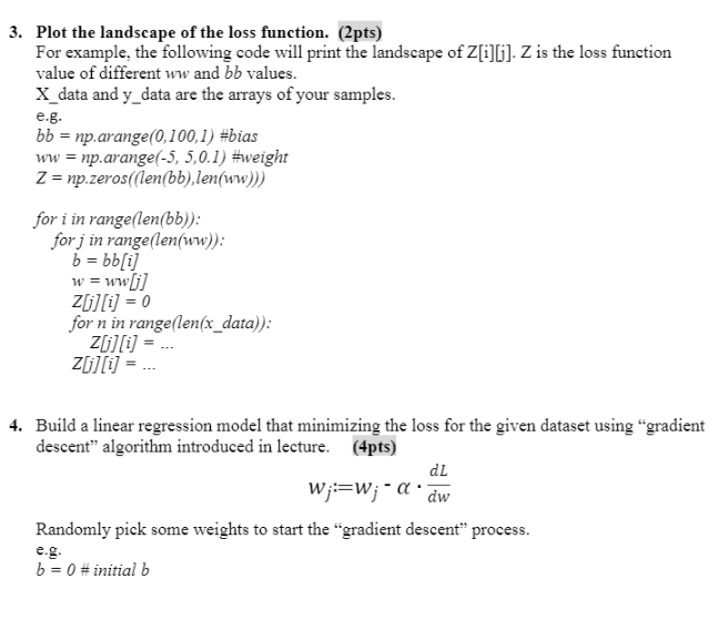
3. Plot the landscape of the loss function. (2pts) For example, the following code will print the landscape of Z[i]G). Z is the loss function value of different ww and bb values. X_data and y_data are the arrays of your samples. e.g. bb = np.arange(0,100,1) #bias ww = np.arange(-5, 5,0.1) #weight Z = np.zeros((len(bb) len(ww))) for i in range(len(bb)): forj in range(len(ww)): b = bb[i] w = ww[i] Z[[i] = 0 for n in range(len(x_data)): 2[i][i] = _ Z[i][i] = ... 4. Build a linear regression model that minimizing the loss for the given dataset using gradient descent" algorithm introduced in lecture. (4pts) dl W;=W; - adw Randomly pick some weights to start the gradient descent" process. b = 0 # initial b w = 0 # initial w Explain how your gradient descent process was terminated (e.g. by testing convergence or finishing certain number of iterations) and explain all threshold values you used in your report. (1pt) 5. Test different values of the learning rate I and different number of iterations/convergence threshold values. Explain how these values affect your program in your report. (1pts) Ir = 0.0001 # example learning rate iteration = 10000 # example iteration number 6. Track the change of the weight values (w and b) from each iteration and plot all the values out. (2pts) #Store parameters for plotting b_history = [b] w_history = [w] #model by gradient descent #... b_history.append(b) w_history.append(w) # plt.plot(b_history, w_history, '.-', ms=3, lw=1.5,color='black') Example track change figure: 2 3 0 -2 40 20 60 80 100 b 3. Plot the landscape of the loss function. (2pts) For example, the following code will print the landscape of Z[i]G). Z is the loss function value of different ww and bb values. X_data and y_data are the arrays of your samples. e.g. bb = np.arange(0,100,1) #bias ww = np.arange(-5, 5,0.1) #weight Z = np.zeros((len(bb) len(ww))) for i in range(len(bb)): forj in range(len(ww)): b = bb[i] w = ww[i] Z[[i] = 0 for n in range(len(x_data)): 2[i][i] = _ Z[i][i] = ... 4. Build a linear regression model that minimizing the loss for the given dataset using gradient descent" algorithm introduced in lecture. (4pts) dl W;=W; - adw Randomly pick some weights to start the gradient descent" process. b = 0 # initial b w = 0 # initial w Explain how your gradient descent process was terminated (e.g. by testing convergence or finishing certain number of iterations) and explain all threshold values you used in your report. (1pt) 5. Test different values of the learning rate I and different number of iterations/convergence threshold values. Explain how these values affect your program in your report. (1pts) Ir = 0.0001 # example learning rate iteration = 10000 # example iteration number 6. Track the change of the weight values (w and b) from each iteration and plot all the values out. (2pts) #Store parameters for plotting b_history = [b] w_history = [w] #model by gradient descent #... b_history.append(b) w_history.append(w) # plt.plot(b_history, w_history, '.-', ms=3, lw=1.5,color='black') Example track change figure: 2 3 0 -2 40 20 60 80 100 b