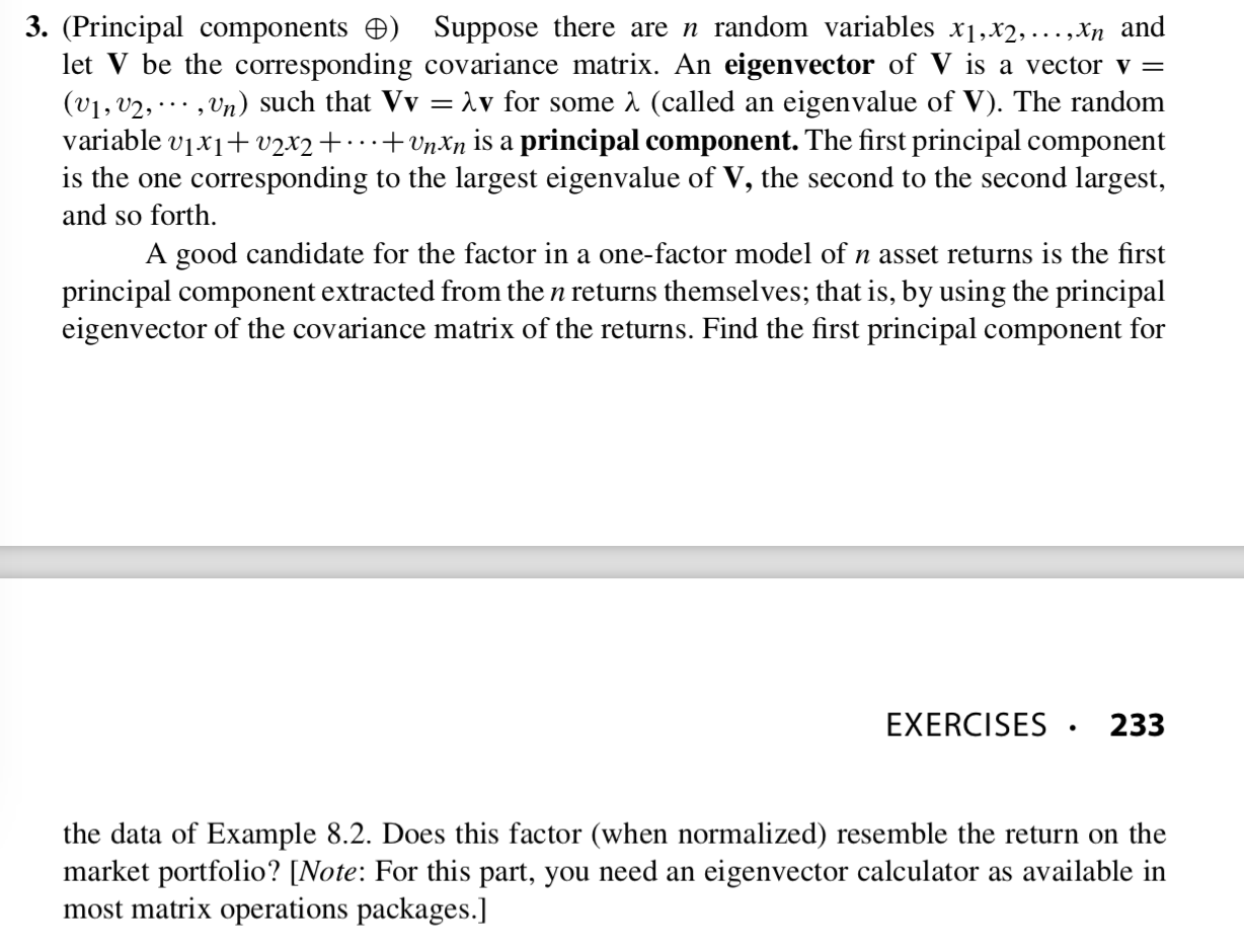
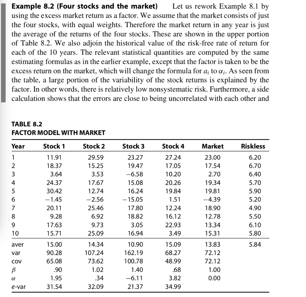
3. (Principal components ) Suppose there are n random variables x1,x2,...,xn and let V be the corresponding covariance matrix. An eigenvector of V is a vector v = (V1, V2, .. , Un) such that Vv = av for some 2 (called an eigenvalue of V). The random variable vixi+ v2x2 +... ... + Unxn is a principal component. The first principal component is the one corresponding to the largest eigenvalue of V, the second to the second largest, and so forth. A good candidate for the factor in a one-factor model of n asset returns is the first principal component extracted from the n returns themselves; that is, by using the principal eigenvector of the covariance matrix of the returns. Find the first principal component for EXERCISES . 233 the data of Example 8.2. Does this factor (when normalized) resemble the return on the market portfolio? [Note: For this part, you need an eigenvector calculator as available in most matrix operations packages.] Example 8.2 (Four stocks and the market) Let us rework Example 8.1 by using the excess market return as a factor. We assume that the market consists of just the four stocks, with equal weights. Therefore the market return in any year is just the average of the returns of the four stocks. These are shown in the upper portion of Table 8.2. We also adjoin the historical value of the risk-free rate of return for each of the 10 years. The relevant statistical quantities are computed by the same estimating formulas as in the earlier example, except that the factor is taken to be the excess return on the market, which will change the formula for a; to Q;. As seen from the table, a large portion of the variability of the stock returns is explained by the factor. In other words, there is relatively low nonsystematic risk. Furthermore, a side calculation shows that the errors are close to being uncorrelated with each other and TABLE 8.2 FACTOR MODEL WITH MARKET Year Stock 1 Stock 2 Stock 3 Stock 4 Market Riskless 1 2 3 4 5 11.91 18.37 3.64 24.37 30.42 -1.45 20.11 9.28 17.63 15.71 29.59 15.25 3.53 17.67 12.74 -2.56 25.46 6.92 9.73 25.09 23.27 19.47 -6.58 15.08 16.24 -15.05 17.80 18.82 3.05 16.94 27.24 17.05 10.20 20.26 19.84 1.51 12.24 16.12 22.93 3.49 23.00 17.54 2.70 19.34 19.81 -4.39 18.90 12.78 13.34 15.31 6.20 6.70 6.40 5.70 5.90 5.20 4.90 5.50 6.10 5.80 6 7 8 9 10 aver 5.84 var 15.00 90.28 65.08 .90 1.95 31.54 14.34 107.24 73.62 1.02 COV B 10.90 162.19 100.78 1.40 -6.11 21.37 15.09 68.27 48.99 .68 3.82 34.99 13.83 72.12 72.12 1.00 0.00 .34 e-var 32.09 3. (Principal components ) Suppose there are n random variables x1,x2,...,xn and let V be the corresponding covariance matrix. An eigenvector of V is a vector v = (V1, V2, .. , Un) such that Vv = av for some 2 (called an eigenvalue of V). The random variable vixi+ v2x2 +... ... + Unxn is a principal component. The first principal component is the one corresponding to the largest eigenvalue of V, the second to the second largest, and so forth. A good candidate for the factor in a one-factor model of n asset returns is the first principal component extracted from the n returns themselves; that is, by using the principal eigenvector of the covariance matrix of the returns. Find the first principal component for EXERCISES . 233 the data of Example 8.2. Does this factor (when normalized) resemble the return on the market portfolio? [Note: For this part, you need an eigenvector calculator as available in most matrix operations packages.] Example 8.2 (Four stocks and the market) Let us rework Example 8.1 by using the excess market return as a factor. We assume that the market consists of just the four stocks, with equal weights. Therefore the market return in any year is just the average of the returns of the four stocks. These are shown in the upper portion of Table 8.2. We also adjoin the historical value of the risk-free rate of return for each of the 10 years. The relevant statistical quantities are computed by the same estimating formulas as in the earlier example, except that the factor is taken to be the excess return on the market, which will change the formula for a; to Q;. As seen from the table, a large portion of the variability of the stock returns is explained by the factor. In other words, there is relatively low nonsystematic risk. Furthermore, a side calculation shows that the errors are close to being uncorrelated with each other and TABLE 8.2 FACTOR MODEL WITH MARKET Year Stock 1 Stock 2 Stock 3 Stock 4 Market Riskless 1 2 3 4 5 11.91 18.37 3.64 24.37 30.42 -1.45 20.11 9.28 17.63 15.71 29.59 15.25 3.53 17.67 12.74 -2.56 25.46 6.92 9.73 25.09 23.27 19.47 -6.58 15.08 16.24 -15.05 17.80 18.82 3.05 16.94 27.24 17.05 10.20 20.26 19.84 1.51 12.24 16.12 22.93 3.49 23.00 17.54 2.70 19.34 19.81 -4.39 18.90 12.78 13.34 15.31 6.20 6.70 6.40 5.70 5.90 5.20 4.90 5.50 6.10 5.80 6 7 8 9 10 aver 5.84 var 15.00 90.28 65.08 .90 1.95 31.54 14.34 107.24 73.62 1.02 COV B 10.90 162.19 100.78 1.40 -6.11 21.37 15.09 68.27 48.99 .68 3.82 34.99 13.83 72.12 72.12 1.00 0.00 .34 e-var 32.09