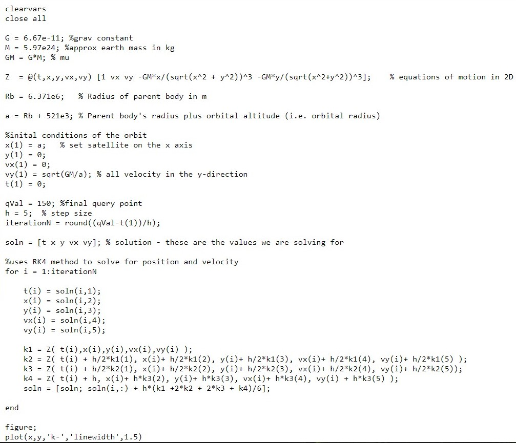
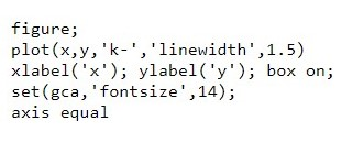
3.2 Part 2 For part 2, begin with a fresh version of RK4_lab_2.m. Here, you are going to plot the trajectory of a Hohmann transfer between two circular orbits. Use a step size of 1 second for this activity. Set the satellite to orbit the Earth at 700 km in a circular orbit, e.g. rc = re + 700 km vy(1) = GM/re . Figure out the time it takes for one orbit. Modify your code so the RK method replaces the position and velocity components at that time to: c(i) = re y(i) = 0 vr(i) = 0 vy(i) = vy(1) + 1800 Increase your Q-val to complete the ellipse . Figure out max and the time at which r == rmar, to get these values you can say: [rMax, MaxIndex) = max(r); in the command window. Modify the code so the RK method replaces the position and velocity components at that time to: x(i) = -Tmax y(i) = 0 vx(i) = 0 vy(i) = - GM/rmax Increase Q-val to complete the new orbit. 7. At what height above Earth's surface is this new orbit? 8. Supply a plot of the trajectory including one orbit in the smaller circular orbit, the transfer and at least one orbit at the new circular radius. 9. Copy and paste your modified code into your lab document. DO NOT SUBMIT YOUR MATLAB SCRIPT TO MOODLE. clearvars close all G = 6.67e-11; %grav constant M = 5.97e24; %approx earth mass in kg GM = G*M; % mu z = @(t,x,y,vx, vy) [1 vx vy -GM*x/(sqrt(x^2 + y^2))^3 -GM*y/(sqrt(x^2+y^2))^3]; % equations of motion in 2D Rb = 6.371e6; % Radius of parent body in m a = Rb + 521e3; % Parent body's radius plus orbital altitude (i.e. orbital radius) %inital conditions of the orbit x(1) = a; % set satellite on the x axis y (1) = 0; vx(1) = 0; vy(1) = sqrt(GM/a); % all velocity in the y-direction t(1) = 0; gVal = 150; %final query point h = 5; % step size iterationN = round((qVal-t(1))/h); soln = [t x y vx vy]; % solution - these are the values we are solving for %uses RK4 method to solve for position and velocity for i = 1:iteration t(i) = soln(i,1); x(i) = soln(i, 2); y(i) = soln(i,3); vx(i) = soln(i, 4); vy(i) = soln(i,5); k1 = z t(i),x(i),y(i), vx(i), vy(i)); k2 = Z( t(i) + h/2*k1(1), x(i)+ h/2*k1(2), y(i)+ h/2*k1(3), vx(i)+ h/2*k1(4), vy(i)+ h/2*k1(5)); k3 = Z( t(i) + h/2*k2(1), x(i)+ h/2*k2(2), y(i)+ h/2*k2(3), vx(i)+ h/2*k2(4), vy(i)+ h/2*k2(5)); k4 = Z( t(i) + h, x(i)+ h*k3(2), y(i)+ h*k3(3), vx(i)+ h*k3(4), vy(i) + h*k3(5)); soln = [soln; soln(i,:) + h* (k1 +2*k2 + 2*k3 + k4)/6]; end figure; plot(x, y, 'k-', 'linewidth',1.5) figure; plot(x,y,'k-', 'linewidth',1.5) xlabel('x'); ylabel('y'); box on; set(gca,'fontsize',14); axis equal 3.2 Part 2 For part 2, begin with a fresh version of RK4_lab_2.m. Here, you are going to plot the trajectory of a Hohmann transfer between two circular orbits. Use a step size of 1 second for this activity. Set the satellite to orbit the Earth at 700 km in a circular orbit, e.g. rc = re + 700 km vy(1) = GM/re . Figure out the time it takes for one orbit. Modify your code so the RK method replaces the position and velocity components at that time to: c(i) = re y(i) = 0 vr(i) = 0 vy(i) = vy(1) + 1800 Increase your Q-val to complete the ellipse . Figure out max and the time at which r == rmar, to get these values you can say: [rMax, MaxIndex) = max(r); in the command window. Modify the code so the RK method replaces the position and velocity components at that time to: x(i) = -Tmax y(i) = 0 vx(i) = 0 vy(i) = - GM/rmax Increase Q-val to complete the new orbit. 7. At what height above Earth's surface is this new orbit? 8. Supply a plot of the trajectory including one orbit in the smaller circular orbit, the transfer and at least one orbit at the new circular radius. 9. Copy and paste your modified code into your lab document. DO NOT SUBMIT YOUR MATLAB SCRIPT TO MOODLE. clearvars close all G = 6.67e-11; %grav constant M = 5.97e24; %approx earth mass in kg GM = G*M; % mu z = @(t,x,y,vx, vy) [1 vx vy -GM*x/(sqrt(x^2 + y^2))^3 -GM*y/(sqrt(x^2+y^2))^3]; % equations of motion in 2D Rb = 6.371e6; % Radius of parent body in m a = Rb + 521e3; % Parent body's radius plus orbital altitude (i.e. orbital radius) %inital conditions of the orbit x(1) = a; % set satellite on the x axis y (1) = 0; vx(1) = 0; vy(1) = sqrt(GM/a); % all velocity in the y-direction t(1) = 0; gVal = 150; %final query point h = 5; % step size iterationN = round((qVal-t(1))/h); soln = [t x y vx vy]; % solution - these are the values we are solving for %uses RK4 method to solve for position and velocity for i = 1:iteration t(i) = soln(i,1); x(i) = soln(i, 2); y(i) = soln(i,3); vx(i) = soln(i, 4); vy(i) = soln(i,5); k1 = z t(i),x(i),y(i), vx(i), vy(i)); k2 = Z( t(i) + h/2*k1(1), x(i)+ h/2*k1(2), y(i)+ h/2*k1(3), vx(i)+ h/2*k1(4), vy(i)+ h/2*k1(5)); k3 = Z( t(i) + h/2*k2(1), x(i)+ h/2*k2(2), y(i)+ h/2*k2(3), vx(i)+ h/2*k2(4), vy(i)+ h/2*k2(5)); k4 = Z( t(i) + h, x(i)+ h*k3(2), y(i)+ h*k3(3), vx(i)+ h*k3(4), vy(i) + h*k3(5)); soln = [soln; soln(i,:) + h* (k1 +2*k2 + 2*k3 + k4)/6]; end figure; plot(x, y, 'k-', 'linewidth',1.5) figure; plot(x,y,'k-', 'linewidth',1.5) xlabel('x'); ylabel('y'); box on; set(gca,'fontsize',14); axis equal