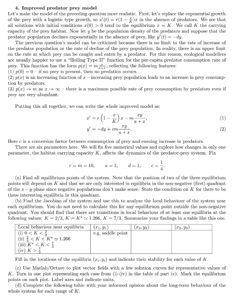
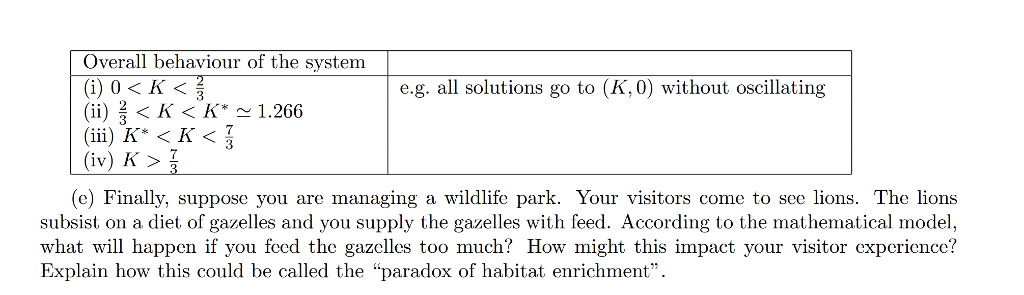
4. Improved predator prey model Let's make the model of the preceding question more realistic. First, let's replace the exponential growth 1 of the prey with a logistic type growth, so z (t) in the absence of predators. We see that all solutions with initial conditions z(0) 0 tend to the equilibrium a K. We call K the carrying capacity of the prey habitat. Now let y be the population density of the predators and suppose that the predator population declines exponentially in the absence of prey, like y dy The previous question's model can be criticized because there is no limit to the rate of increase of the predator population or the rate of decline of the prey population. In reality, there is an upper limit on the rate at which prey can be caught and eaten by a predator. For this reason, ecological modellers are usually happier to use a "Holling Type II" function for the per-capita predator consumption rate of prey. This function has the form p reflecting the following features (1) p (0) -0 f no prey is present, then no predation occurs (2) p(ar) is an increasing function of increasing prey population leads to an increase in prey consump- ion by predators (3) p(ar) m as a co there is a maximum possible rate of prey consumption by predators even if prey are very abundant Putting this all together, we can write the whole improved model as: (1) r 1 (2) dy cm Here c is a conversion factor between consumption of prey and ensuing increase in predators There are six parameters here. We will fix five numerical values and explore how changes in only one parameter, the habitat carrying capacity K, affects the dynamics of the predator-prey system. Fix 10 (a) Find all equilibrium points of the system. Note that the position of two of the three equilibrium points will depend on K and that we are only interested in equilibria in the non-negative (first) quadrant of the z-y plane since negative populations don't make sense. State the condition on K for there to be three interesting equilibria in this quadrant (b) Find the Jacobian of the system and use this to analyze the local behaviour of the system near each equilibrium. You do not need to calculate this for any equilibrium point outside the non-megative quadrant. You should find that there are transitions in local behaviour of at least one equilibria at the /3, K K 1.266, K 7/3. Summarize your findings in a table like this one following values: K Local haviour near equilibria yl (72, T3, g. Saddle poin ii) K K 1.266 iii) K* K Fill in the locations of the equilibria (ri, yi) and indicate their stability for each value of K (c) Use Matlab Octave to plot vector fields with a few solution curves for representative values of Civ) in the table of part (c). Mark the equilibrium K. Turn in one plot representing each case from (i points on each Label plot. axes and indicate units (d) Complete the following table with your informed opinion about the long-term behaviour of the whole system for each range of K 4. Improved predator prey model Let's make the model of the preceding question more realistic. First, let's replace the exponential growth 1 of the prey with a logistic type growth, so z (t) in the absence of predators. We see that all solutions with initial conditions z(0) 0 tend to the equilibrium a K. We call K the carrying capacity of the prey habitat. Now let y be the population density of the predators and suppose that the predator population declines exponentially in the absence of prey, like y dy The previous question's model can be criticized because there is no limit to the rate of increase of the predator population or the rate of decline of the prey population. In reality, there is an upper limit on the rate at which prey can be caught and eaten by a predator. For this reason, ecological modellers are usually happier to use a "Holling Type II" function for the per-capita predator consumption rate of prey. This function has the form p reflecting the following features (1) p (0) -0 f no prey is present, then no predation occurs (2) p(ar) is an increasing function of increasing prey population leads to an increase in prey consump- ion by predators (3) p(ar) m as a co there is a maximum possible rate of prey consumption by predators even if prey are very abundant Putting this all together, we can write the whole improved model as: (1) r 1 (2) dy cm Here c is a conversion factor between consumption of prey and ensuing increase in predators There are six parameters here. We will fix five numerical values and explore how changes in only one parameter, the habitat carrying capacity K, affects the dynamics of the predator-prey system. Fix 10 (a) Find all equilibrium points of the system. Note that the position of two of the three equilibrium points will depend on K and that we are only interested in equilibria in the non-negative (first) quadrant of the z-y plane since negative populations don't make sense. State the condition on K for there to be three interesting equilibria in this quadrant (b) Find the Jacobian of the system and use this to analyze the local behaviour of the system near each equilibrium. You do not need to calculate this for any equilibrium point outside the non-megative quadrant. You should find that there are transitions in local behaviour of at least one equilibria at the /3, K K 1.266, K 7/3. Summarize your findings in a table like this one following values: K Local haviour near equilibria yl (72, T3, g. Saddle poin ii) K K 1.266 iii) K* K Fill in the locations of the equilibria (ri, yi) and indicate their stability for each value of K (c) Use Matlab Octave to plot vector fields with a few solution curves for representative values of Civ) in the table of part (c). Mark the equilibrium K. Turn in one plot representing each case from (i points on each Label plot. axes and indicate units (d) Complete the following table with your informed opinion about the long-term behaviour of the whole system for each range of K