4) Please solve asap

please solve ASAP

4:

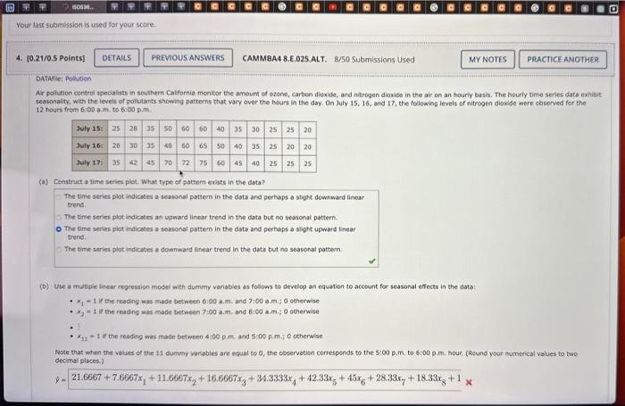
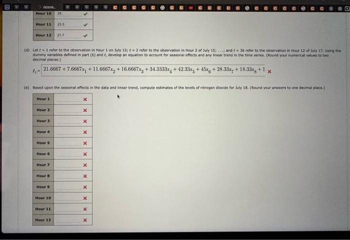
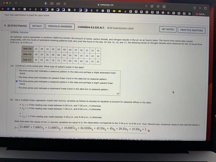
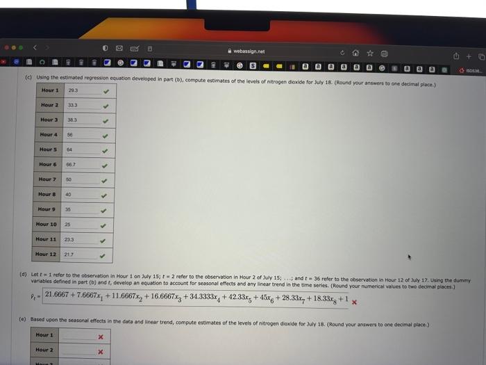
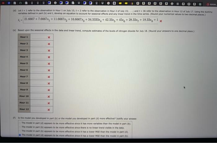
Ar polution control ppecalitts in southem Calfomia monitor the ampunt of szone, carbon dioxide, and nitrogen diaxide in the air on an houriy basis. The hourly time series date exhibit seasonality, with the levels of polutants showing patterns that vary over the heurs in the day. On July 15, 16, aed 17, the following levels of nitrogen dioside were coserved for the 12 haurs frem 6.00 a.m. to 6.00 p.m. (a) Censtruct a time series plot. What type of pattern exists in the data? The time series plot indicates a seasonal pattem in the dsts and perhaps a sight dowriward linear trent. The timie series plot indicates an upward linear trend in the data but no seasonat pattem. The time series plat inticates a seasonal pattem in the data and pertaps a sloht upward inear trend. The time series plot indicates a downward linear trend in the dats but no seasonal pottem. (b) Use a mubpie linear regression modei with dummy variables as folliws to develop an equation to ateount for seasonal effects in the data: - x11 if the reeding was made between 6:00 a,m. and 7:00 am.; 0 otherwise - x2= if the reading was made between 7:00 a.m. and b tio 00 am, 0 atherwise. - x11=1 if the reading was made between 4:00p.m, and 5:00p.m.40 ocherwise Note that when the vatues of the 11 dummy varabies are equal to 0 , the observabisa correspends to the 5:00 p.m. to 6:00 p.m. Bour. (Re4nd your eumerical values to two decinal places.) x^=21.6667+7.6667x1+11.6667x2+16.6667x3+34.3333x4+42.33x5+45x6+28.33x7+18.33x8+1x3 (d) Let t=1 refer to the observation in Hour 1 on July 15;t=2 refer to the observatien in Hour 2 of July 15;...4 and t=36 refer to the observation in Hour 12 of zuly 17 . Using the dummy variables defined in part (b) and t, develop an equation to account for seasonal effects and any linear trend in the time series. (Reund your numerical values to two decimal places.) t=21.6667+7.6667x1+11.6667x2+16.6667x3+34.3333x4+42.33x5+45x6+28.33x7+18.33x8+1 (a) Construct a bitre series plot. What type of pattem exists in the data? The time series plot indicates a seasonal pattern in the data and perhaps a slight downsard linear trend. The time series plot incicates an upward linear trend in the data but no stasonal pattern, The sime series plot indicates a sessonal pattem in the dats and perhaps a silght voward inear trend. The tine series plot indicates a downward linear trend in the data but no sessonal pottern. (b) Use a mutiple linear regression model with dumny variasles as follows to efvelop an equation to account for seasenal effects in the data: - x1=1 if the roading was made between 6:00am, and 7:00 a.m.; 0 otherwise +. x2=1 it the reading was made between 7:00 a.m, and 8:00 a.m, 0 otherwise - x141 ir the reading was mode between 4:00 p.m. and 5:00 p.m,; 0 otherwise Note that ehen the veleses of the 11 dummy variables are equil to 0 , the observation cocresponds to the 5:00 p.m. to 6:00 p.m. hour (hound your numerical values to two tecimal places 3 y=21.6667+7.6667x1+11.6667x2+16.6667x3+34.3333x4+42.33x5+45x6+28.33x7+18.33x8+1x8 Let t=1 refer to the observation in Hour 1 on July 15;t=2 reter to the observation in Hour 2 of July 15; i . ; and t=36 refer to the observation in Hour 12 of lay 17 . Using the duminy variables defined in part (b) and tr develop an equation to account for seasonal effects and any linear trend in the time series. (Reund vour numenkal values to two decimat places.) t=21.6667+7.6667x1+11.6667x2+16.6667x3+34.3333x4+42.33x5+45x6+28.33x7+18.33x8+1x7 (d) Let t=1 mefer to the observation in Hour 1 on July 15;t=2 refer to the observation in Hour 2 of Zuly 15 ; ...i; and t=36 refer to the observation in Hour 12 of July 17 . Using the duntmy: velabies defined in part (b) and t, develop an equation to account for seasonal effects and any linear trend in the sime series. (Round your numerical values to two decimal places ) ^t=21.6667+7.6667x1+11.6667x2+16.6667x3+34.3333x4+42.33x5+45x6+28.33x7+18.33x8+1x3 (e) (1) Is the model you developed in part (b) or the model you devsleped in part (d) mere effective? kustify your answer. The model in part (d) appears to be mese effeceive eince is hes more varlables than the model in 0 art (b). The madel in part (b) appears to be more effective coce there is no linear trend vibible in the deta. The modet in part (b) oppears to be msere effective since it has a lower Mas itan the model in part (d). The Thodet in pat (d) appears 6 be more effective vhre it has a lower Maf than the moset in part (b). Ar polution control ppecalitts in southem Calfomia monitor the ampunt of szone, carbon dioxide, and nitrogen diaxide in the air on an houriy basis. The hourly time series date exhibit seasonality, with the levels of polutants showing patterns that vary over the heurs in the day. On July 15, 16, aed 17, the following levels of nitrogen dioside were coserved for the 12 haurs frem 6.00 a.m. to 6.00 p.m. (a) Censtruct a time series plot. What type of pattern exists in the data? The time series plot indicates a seasonal pattem in the dsts and perhaps a sight dowriward linear trent. The timie series plot indicates an upward linear trend in the data but no seasonat pattem. The time series plat inticates a seasonal pattem in the data and pertaps a sloht upward inear trend. The time series plot indicates a downward linear trend in the dats but no seasonal pottem. (b) Use a mubpie linear regression modei with dummy variables as folliws to develop an equation to ateount for seasonal effects in the data: - x11 if the reeding was made between 6:00 a,m. and 7:00 am.; 0 otherwise - x2= if the reading was made between 7:00 a.m. and b tio 00 am, 0 atherwise. - x11=1 if the reading was made between 4:00p.m, and 5:00p.m.40 ocherwise Note that when the vatues of the 11 dummy varabies are equal to 0 , the observabisa correspends to the 5:00 p.m. to 6:00 p.m. Bour. (Re4nd your eumerical values to two decinal places.) x^=21.6667+7.6667x1+11.6667x2+16.6667x3+34.3333x4+42.33x5+45x6+28.33x7+18.33x8+1x3 (d) Let t=1 refer to the observation in Hour 1 on July 15;t=2 refer to the observatien in Hour 2 of July 15;...4 and t=36 refer to the observation in Hour 12 of zuly 17 . Using the dummy variables defined in part (b) and t, develop an equation to account for seasonal effects and any linear trend in the time series. (Reund your numerical values to two decimal places.) t=21.6667+7.6667x1+11.6667x2+16.6667x3+34.3333x4+42.33x5+45x6+28.33x7+18.33x8+1 (a) Construct a bitre series plot. What type of pattem exists in the data? The time series plot indicates a seasonal pattern in the data and perhaps a slight downsard linear trend. The time series plot incicates an upward linear trend in the data but no stasonal pattern, The sime series plot indicates a sessonal pattem in the dats and perhaps a silght voward inear trend. The tine series plot indicates a downward linear trend in the data but no sessonal pottern. (b) Use a mutiple linear regression model with dumny variasles as follows to efvelop an equation to account for seasenal effects in the data: - x1=1 if the roading was made between 6:00am, and 7:00 a.m.; 0 otherwise +. x2=1 it the reading was made between 7:00 a.m, and 8:00 a.m, 0 otherwise - x141 ir the reading was mode between 4:00 p.m. and 5:00 p.m,; 0 otherwise Note that ehen the veleses of the 11 dummy variables are equil to 0 , the observation cocresponds to the 5:00 p.m. to 6:00 p.m. hour (hound your numerical values to two tecimal places 3 y=21.6667+7.6667x1+11.6667x2+16.6667x3+34.3333x4+42.33x5+45x6+28.33x7+18.33x8+1x8 Let t=1 refer to the observation in Hour 1 on July 15;t=2 reter to the observation in Hour 2 of July 15; i . ; and t=36 refer to the observation in Hour 12 of lay 17 . Using the duminy variables defined in part (b) and tr develop an equation to account for seasonal effects and any linear trend in the time series. (Reund vour numenkal values to two decimat places.) t=21.6667+7.6667x1+11.6667x2+16.6667x3+34.3333x4+42.33x5+45x6+28.33x7+18.33x8+1x7 (d) Let t=1 mefer to the observation in Hour 1 on July 15;t=2 refer to the observation in Hour 2 of Zuly 15 ; ...i; and t=36 refer to the observation in Hour 12 of July 17 . Using the duntmy: velabies defined in part (b) and t, develop an equation to account for seasonal effects and any linear trend in the sime series. (Round your numerical values to two decimal places ) ^t=21.6667+7.6667x1+11.6667x2+16.6667x3+34.3333x4+42.33x5+45x6+28.33x7+18.33x8+1x3 (e) (1) Is the model you developed in part (b) or the model you devsleped in part (d) mere effective? kustify your answer. The model in part (d) appears to be mese effeceive eince is hes more varlables than the model in 0 art (b). The madel in part (b) appears to be more effective coce there is no linear trend vibible in the deta. The modet in part (b) oppears to be msere effective since it has a lower Mas itan the model in part (d). The Thodet in pat (d) appears 6 be more effective vhre it has a lower Maf than the moset in part (b)