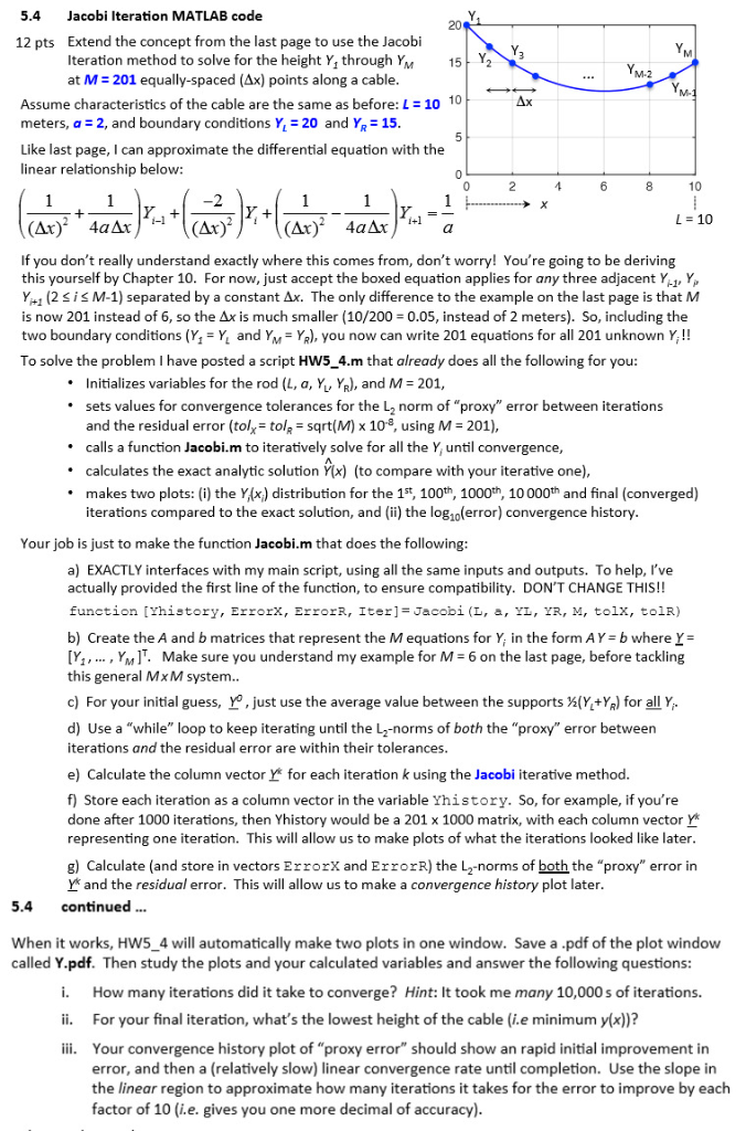
5.4 Jacobi Iteration MATLAB code Extend the concept from the last page to use the Jacobi Iteration method to solve for the height Y, through YM at M-201 equally-spaced (Ax) points along a cable 20 12 pts 15 12 Assume characteristics of the cable are the same as before: L 10 10 meters, a 2, and boundary conditions Y20 and YR 15 Like last page, I can approximate the differential equation with the linear relationship below: i+1 L- 10 (Ar)" 4aAr (Ar) (" 4aAr If you don't really understand exactly where this comes from, don't worry! You're going to be deriving this yourself by Chapter 10. For now, just accept the boxed equation applies for any three adjacent Y, Y y,1 (25 i M-1) separated by a constant . The only difference to the example on the last page is that M is now 201 instead of 6, so the Ax is much smaller (10/200-0.05, instead of 2 meters). So, including the two boundary conditions (Y Y and YM YR), you now can write 201 equations for all 201 unknown Y,!! To solve the problem I have posted a script HW5 4.m that already does all the following for you Initializes variables for the rod (L, a, sets values for convergence tolerances for the L2 norm of "proxy" error between iterations and the residual error toto sqrt(M) x 108, using M-201), calls a function Jacobi.m to iteratively solve for all the Y, until convergence %), and M-201, . " calculates the exact analytic solution Y(x) to compare with your iterative one) makes two plots: (i) the Y(x) distribution for the 1st, 100th, 1000th, 10 000th and final (converged) iterations compared to the exact solution, and (i) the log1o(error) convergence history Your job is just to make the function Jacobi.m that does the following a) EXACTLY interfaces with my main script, using all the same inputs and outputs. To help, I've actually provided the first line of the function, to ensure compatibility. DON'T CHANGE THIS!! function [Yhistory, Errorx, ErrorR, Iterl Jacobi (L, a, YL, R, M, tolx, tolR) b) Create the A and b matrices that represent the M equations for, in the form A Y-b where r= [Y, , Yn Make sure you understand my example for M-6 on the last page, before tackling this general MxM system.. c) For your initial guess, yo, just use the average value between the supports M+%) for all Y. d) Use a "while" loop to keep iterating until the L2-norms of both the "proxy" error between iterations and the residual error are within their tolerances e) Calculate the column vector for each iteration k using the Jacobi iterative methood f) Store each iteration as a column vector in the variable Yhistory. So, for example, if you're done after 1000 iterations, then Yhistory would be a 201 x 1000 matrix, with each column vector Y representing one iteration. This will allow us to make plots of what the iterations looked like later g) Calculate (and store in vectors ErrorX and ErrorR) the L2-norms of both the "proxy" error in Y and the residual error. This will allow us to make a convergence history plot later 5.4 continued.. When it works, HW5_4 will automatically make two plots in one window. Save a .pdf of the plot window called Y.pdf. Then study the plots and your calculated variables and answer the following questions: i. How many iterations did it take to converge? Hint: It took me many 10,000s of iterations. ii. For your final iteration, what's the lowest height of the cable (i.e minimum y(x))? ii Your convergence history plot of "proxy error" should show an rapid initial improvement in error, and then a (relatively slow) linear convergence rate until completion. Use the slope in the linear region to approximate how many iterations it takes for the error to improve by each factor of 10 (i.e. gives you one more decimal of accuracy) 5.4 Jacobi Iteration MATLAB code Extend the concept from the last page to use the Jacobi Iteration method to solve for the height Y, through YM at M-201 equally-spaced (Ax) points along a cable 20 12 pts 15 12 Assume characteristics of the cable are the same as before: L 10 10 meters, a 2, and boundary conditions Y20 and YR 15 Like last page, I can approximate the differential equation with the linear relationship below: i+1 L- 10 (Ar)" 4aAr (Ar) (" 4aAr If you don't really understand exactly where this comes from, don't worry! You're going to be deriving this yourself by Chapter 10. For now, just accept the boxed equation applies for any three adjacent Y, Y y,1 (25 i M-1) separated by a constant . The only difference to the example on the last page is that M is now 201 instead of 6, so the Ax is much smaller (10/200-0.05, instead of 2 meters). So, including the two boundary conditions (Y Y and YM YR), you now can write 201 equations for all 201 unknown Y,!! To solve the problem I have posted a script HW5 4.m that already does all the following for you Initializes variables for the rod (L, a, sets values for convergence tolerances for the L2 norm of "proxy" error between iterations and the residual error toto sqrt(M) x 108, using M-201), calls a function Jacobi.m to iteratively solve for all the Y, until convergence %), and M-201, . " calculates the exact analytic solution Y(x) to compare with your iterative one) makes two plots: (i) the Y(x) distribution for the 1st, 100th, 1000th, 10 000th and final (converged) iterations compared to the exact solution, and (i) the log1o(error) convergence history Your job is just to make the function Jacobi.m that does the following a) EXACTLY interfaces with my main script, using all the same inputs and outputs. To help, I've actually provided the first line of the function, to ensure compatibility. DON'T CHANGE THIS!! function [Yhistory, Errorx, ErrorR, Iterl Jacobi (L, a, YL, R, M, tolx, tolR) b) Create the A and b matrices that represent the M equations for, in the form A Y-b where r= [Y, , Yn Make sure you understand my example for M-6 on the last page, before tackling this general MxM system.. c) For your initial guess, yo, just use the average value between the supports M+%) for all Y. d) Use a "while" loop to keep iterating until the L2-norms of both the "proxy" error between iterations and the residual error are within their tolerances e) Calculate the column vector for each iteration k using the Jacobi iterative methood f) Store each iteration as a column vector in the variable Yhistory. So, for example, if you're done after 1000 iterations, then Yhistory would be a 201 x 1000 matrix, with each column vector Y representing one iteration. This will allow us to make plots of what the iterations looked like later g) Calculate (and store in vectors ErrorX and ErrorR) the L2-norms of both the "proxy" error in Y and the residual error. This will allow us to make a convergence history plot later 5.4 continued.. When it works, HW5_4 will automatically make two plots in one window. Save a .pdf of the plot window called Y.pdf. Then study the plots and your calculated variables and answer the following questions: i. How many iterations did it take to converge? Hint: It took me many 10,000s of iterations. ii. For your final iteration, what's the lowest height of the cable (i.e minimum y(x))? ii Your convergence history plot of "proxy error" should show an rapid initial improvement in error, and then a (relatively slow) linear convergence rate until completion. Use the slope in the linear region to approximate how many iterations it takes for the error to improve by each factor of 10 (i.e. gives you one more decimal of accuracy)