Any help with this code would be of great help, especially D through G.

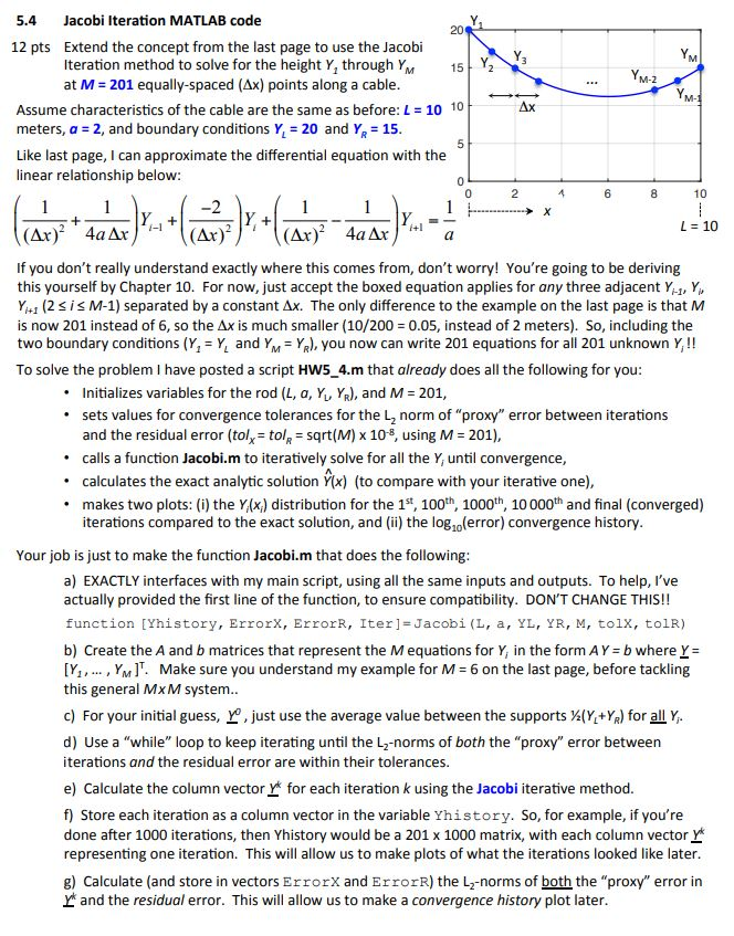
5.4 Jacobi Iteration MATLAB code 20 12 pts Extend the concept from the last page to use the Jacobi Iteration method to solve for the height Y, through Yw at M 201 equally-spaced (Ax) points along a cable 15 2 M-2 Assume characteristics of the cable are the same as before: L 10 10 meters, a-2, and boundary conditions Y 20 and YR 15 Like last page, I can approximate the differential equation with the linear relationship below 0 2 10 (mF.al. .(j)r.( ) L 10 (Ar)- 4a Ar (Ar)2 4a Ar If you don't really understand exactly where this comes from, don't worry! You're going to be deriving this yourself by Chapter 10. For now, just accept the boxed equation applies for any three adjacent Y-1, y,1 (2 i M-1) separated by a constant Ax. The only difference to the example on the last page is that M is now 201 instead of 6, so the is much smaller (10/200 = 0.05, instead of 2 meters). So, including the two boundary conditions (Y,-, and Yn-YR), you now can write 201 equations for all 201 unknown Y!! To solve the problem I have posted a script HW5 4.m that already does all the following for you Initializes variables for the rod (L, a, Yu YR), and M = 201 sets values for convergence tolerances for the L2 norm of "proxy" error between iterations and the residual error (tol,-tol,-sqrt(M) x 108, using M = 201) . calls a function Jacobi.m to iteratively solve for all the Y, until convergence calculates the exact analytic solution Y(x) (to compare with your iterative one) makes two plots: (i) the Y(x) distribution for the 1st, 100th, 100oth, 10 000th and final (converged) iterations compared to the exact solution, and (ii) the log(error) convergence history Your job is just to make the function Jacobi.m that does the following a) EXACTLY interfaces with my main script, using all the same inputs and outputs. To help, I've actually provided the first line of the function, to ensure compatibility. DON'T CHANGE THIS!! function [Yhistory, Errorx, ErrorR, Iter] Jacobi (L, a, YL, YR, M, tolx, tolR) b) Create the A and b matrices that represent the M equations for Y, in the form A Y# b where Y: [Yn , Yna ]T. Make sure you understand my example for M = 6 on the last page, before tackling this general Mx M system c) For your initial guess, r, just use the average value between the supports (+%) for all Y. d) Use a "while" loop to keep iterating until the L2-norms of both the "proxy" error between iterations and the residual error are within their tolerances. e) Calculate the column vector x for each iteration k using the Jacobi iterative method f Store each iteration as a column vector in the variable Yhistory. So, for example, if you're done after 1000 iterations, then Yhistory would be a 201 x 1000 matrix, with each column vector Y representing one iteration. This will allow us to make plots of what the iterations looked like later g) Calculate (and store in vectors Errorx and ErrorR) the L2-norms of both the "proxy" error in Yand the residual error. This will allow us to make a convergence history plot later. 5.4 Jacobi Iteration MATLAB code 20 12 pts Extend the concept from the last page to use the Jacobi Iteration method to solve for the height Y, through Yw at M 201 equally-spaced (Ax) points along a cable 15 2 M-2 Assume characteristics of the cable are the same as before: L 10 10 meters, a-2, and boundary conditions Y 20 and YR 15 Like last page, I can approximate the differential equation with the linear relationship below 0 2 10 (mF.al. .(j)r.( ) L 10 (Ar)- 4a Ar (Ar)2 4a Ar If you don't really understand exactly where this comes from, don't worry! You're going to be deriving this yourself by Chapter 10. For now, just accept the boxed equation applies for any three adjacent Y-1, y,1 (2 i M-1) separated by a constant Ax. The only difference to the example on the last page is that M is now 201 instead of 6, so the is much smaller (10/200 = 0.05, instead of 2 meters). So, including the two boundary conditions (Y,-, and Yn-YR), you now can write 201 equations for all 201 unknown Y!! To solve the problem I have posted a script HW5 4.m that already does all the following for you Initializes variables for the rod (L, a, Yu YR), and M = 201 sets values for convergence tolerances for the L2 norm of "proxy" error between iterations and the residual error (tol,-tol,-sqrt(M) x 108, using M = 201) . calls a function Jacobi.m to iteratively solve for all the Y, until convergence calculates the exact analytic solution Y(x) (to compare with your iterative one) makes two plots: (i) the Y(x) distribution for the 1st, 100th, 100oth, 10 000th and final (converged) iterations compared to the exact solution, and (ii) the log(error) convergence history Your job is just to make the function Jacobi.m that does the following a) EXACTLY interfaces with my main script, using all the same inputs and outputs. To help, I've actually provided the first line of the function, to ensure compatibility. DON'T CHANGE THIS!! function [Yhistory, Errorx, ErrorR, Iter] Jacobi (L, a, YL, YR, M, tolx, tolR) b) Create the A and b matrices that represent the M equations for Y, in the form A Y# b where Y: [Yn , Yna ]T. Make sure you understand my example for M = 6 on the last page, before tackling this general Mx M system c) For your initial guess, r, just use the average value between the supports (+%) for all Y. d) Use a "while" loop to keep iterating until the L2-norms of both the "proxy" error between iterations and the residual error are within their tolerances. e) Calculate the column vector x for each iteration k using the Jacobi iterative method f Store each iteration as a column vector in the variable Yhistory. So, for example, if you're done after 1000 iterations, then Yhistory would be a 201 x 1000 matrix, with each column vector Y representing one iteration. This will allow us to make plots of what the iterations looked like later g) Calculate (and store in vectors Errorx and ErrorR) the L2-norms of both the "proxy" error in Yand the residual error. This will allow us to make a convergence history plot later