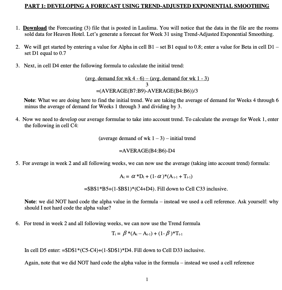
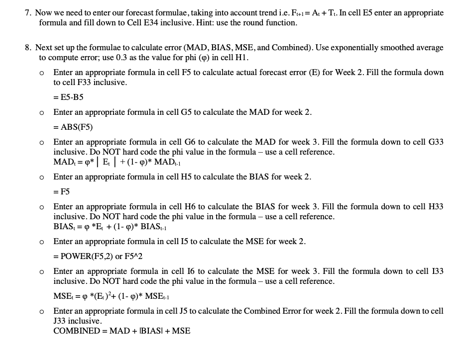
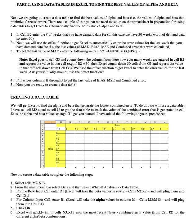
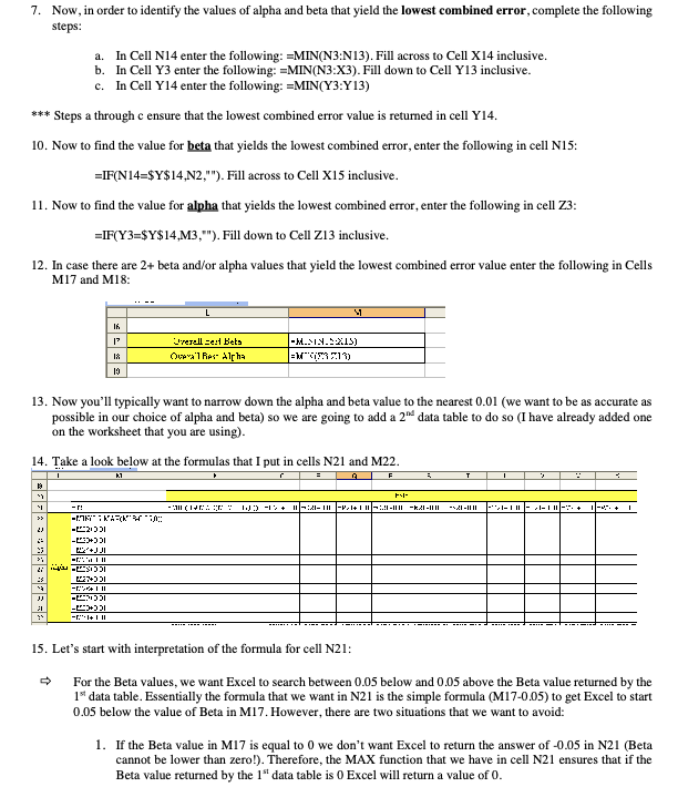
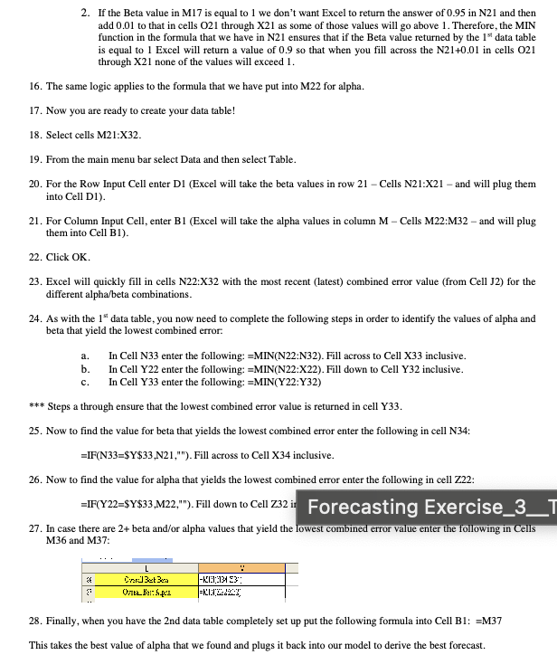
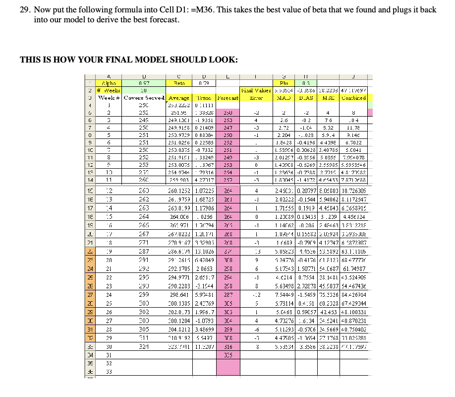
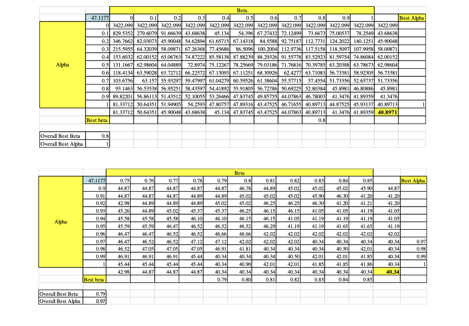
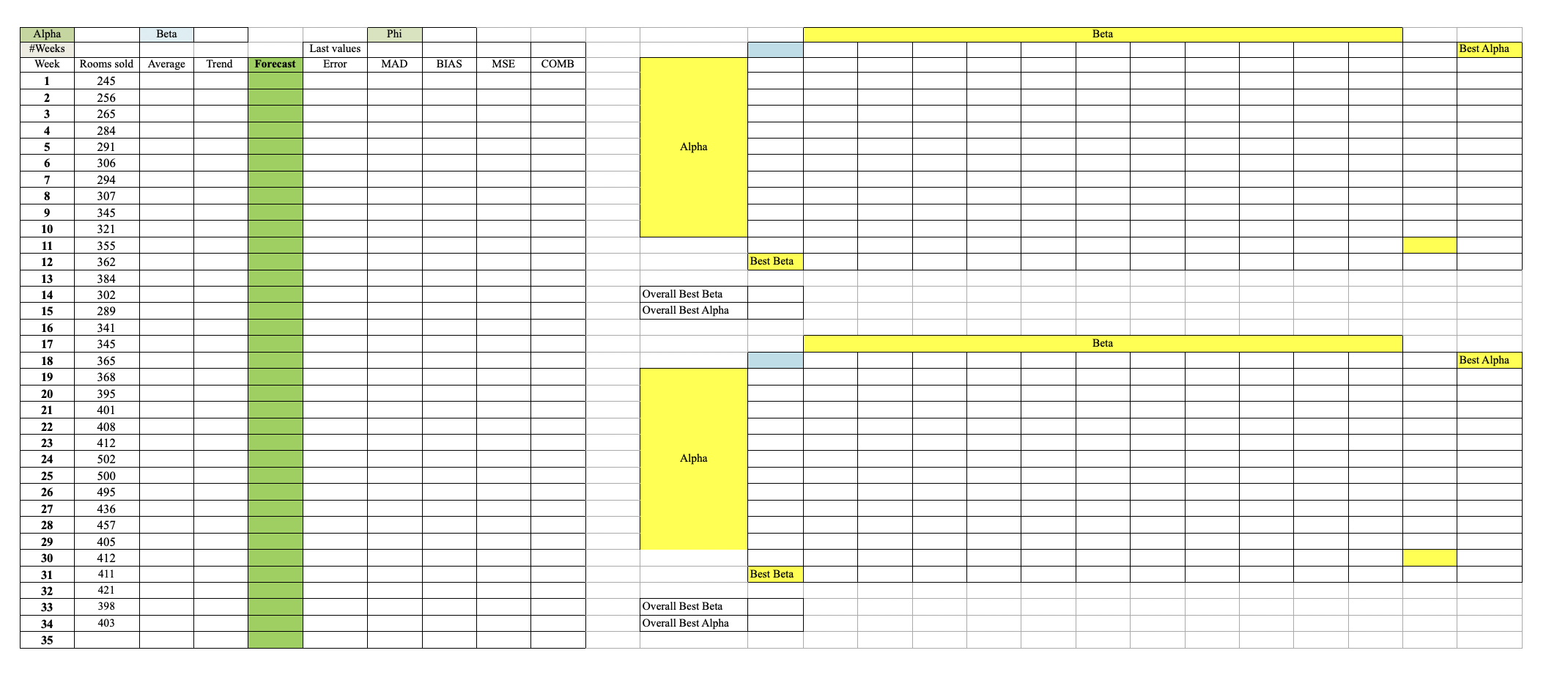
6. PART 1: DEVELOPING A FORECAST USING TREND-ADJUSTED EXPONENTIAL SMOOTHING Download the Forecasting (3) file that is posted in Laulima. You will notice that the data in the file are the rooms sold data for Heaven Hotel. Let's generate a forecast for Week 31 using Trend-Adjusted Exponential Smoothing. . We will get started by entering a value for Alpha in cell B1 set B1 equal to 0.8; enter a value for Beta in cell Dl set D1 equal to 0.7 . Next, in cell D4 enter the following formula to calculate the initial trend: (avg. demand for wk 4 - 6) (avg. demand for wk 1 - 3) 3 =(A VER AGE(B7:B9)-A VERAGE(B4:B6))/3 Note: What we are doing here to find the initial trend. We are taking the average of demand for Weeks 4 through 6 minus the average of demand for Weeks 1 through 3 and dividing by 3. . Now we need to develop our average formulae to take into account trend. To calculate the average for Week 1, enter the following in cell C4: (average demand of wk | 3) initial trend =AVERAGE(B4:B6)-D4 . For average in week 2 and all following weeks, we can now use the average (taking into account trend) formula: Ac= @ *D, + (1-@ )*(Aci + Te) =$B$1*B5+(1-$B$1)*(C4+D4). Fill down to Cell C33 inclusive. Note: we did NOT hard code the alpha value in the formula instead we used a cell reference. Ask yourself: why should I not hard code the alpha value? For trend in week 2 and all following weeks, we can now use the Trend formula Tr= 8 *(Ac Aci) + (1-8 )*Te In cell D5 enter: =$D$1*(C5-C4)+(1-$D$1)*D4. Fill down to Cell D33 inclusive. Again, note that we did NOT hard code the alpha value in the formula instead we used a cell reference 7. Now we need to enter our forecast formulae, taking into account trend i.e. Fiui= Ar+T:. In cell ES enter an appropriate formula and fill down to Cell E34 inclusive. Hint: use the round function. 8. Next set up the formulae to calculate error (MAD, BIAS, MSE, and Combined). Use exponentially smoothed average to compute error; use 0.3 as the value for phi (@) in cell H1. Oo Enter an appropriate formula in cell F5 to calculate actual forecast error (E) for Week 2. Fill the formula down to cell F33 inclusive. = E5-B5 Enter an appropriate formula in cell G5 to calculate the MAD for week 2. = ABS(F5) Enter an appropriate formula in cell G6 to calculate the MAD for week 3. Fill the formula down to cell G33 inclusive. Do NOT hard code the phi value in the formula use a cell reference. MAD,= 9*| E, | +(1-9)* MAD. Enter an appropriate formula in cell H5 to calculate the BIAS for week 2. =F5 Enter an appropriate formula in cell H6 to calculate the BLAS for week 3. Fill the formula down to cell H33 inclusive. Do NOT hard code the phi value in the formula use a cell reference. BIAS, = 9 *E, + (1- 9)* BIAS,; Enter an appropriate formula in cell IS to calculate the MSE for week 2. = POWER(F5S,2) or F542 Enter an appropriate formula in cell I6 to calculate the MSE for week 3. Fill the formula down to cell 133 inclusive. Do NOT hard code the phi value in the formula use a cell reference. MSE. = 9 *(E:)'+ (1- 9)* MSE:1 Enter an appropriate formula in cell J5 to calculate the Combined Error for week 2. Fill the formula down to cell J33 inclusive. COMBINED = MAD + IBIAS! + MSE Next we are going to create a data table to find the best values of alpha and beta (i.e. the values of alpha and beta that mninimize forecast error). There are a couple of things that we need to set up on the spreadsheet in preparation for using data tables to get Excel to automatically find the best value of alpha and beta: 2. In Cell B2 enter the # of weeks that you have demand data for (In this case we have 30 weeks worth of demand data so enter 30) Next, we will use the offset function to get Excel to automatically enter the error values for the last week that you have demand data for (i.e. the last values of MAD, BLAS, MSE and Combined error that were calculated) To get the last value of MAD enter the following in Cell G2: =OFFSET(G3,$B$2,0) Note: Excel goes to cell G3 and counts down the column from there how ever many weeks are entered in cell BZ and reports the value in that cell (e.g. if B2 = 30, then Excel counts down 30 cells from G3 and reports the value in that 30 cell down from Cell G3). We used the offset function to get Excel to enter the error values for the last week. Ask yourself: why should I use the offset function? Fill across columns H through J to get the last value of BLAS, MSE and Combined error. Now you are ready to create a data table! CREATING A DATA TABLE: We will get Excel to find the alpha and beta that generate the lowest combined error. To do this we will use a data table. I have set cell M2 equal to cell J2 to get the data table to track the value of the combined error that is generated in cell J2 as the alpha and beta values change. To get you started, I have added the following to your spreadsheet: ic Mi 4 a a 3 Beta as T u ca We a2 0.3 a? Now, to create a data table complete the following steps: a be - Select cells M2:X13. . From the main menu bar select Data and then select What-If Analysis - Data Table. For the Row Input Cell enter D1 (Excel will take the beta values in row 2 Cells N2:X2 and will plug them into Cell D1) For Column Input Cell, enter B! (Excel will take the alpha values in column M = Cells M3:M13 = and will plug them into Cell BI) Click OK. Excel will quickly fill in cells N3:X13 with the most recent (latest) combined error value (from Cell J2) for the different alpha/beta combinations. 7. Now, in order to identify the values of alpha and beta that yield the lowest combined error, complete the following steps: a. In Cell N14 enter the following: =MIN(N3:N13). Fill across to Cell X14 inclusive. b. In Cell Y3 enter the following: =MIN(N3:X3). Fill down to Cell Y13 inclusive. c. In Cell Y14 enter the following: =MIN(Y3:Y13) ***Steps a through c ensure that the lowest combined error value is returned in cell Y14. 10. Now to find the value for beta that yields the lowest combined error, enter the following in cell N15: =IF(N14=$Y$14,N2,""). Fill across to Cell X15 inclusive. 11. Now to find the value for alpha that yields the lowest combined error, enter the following in cell Z3: =IF(Y3=$Y$14,M3,"). Fill down to Cell 213 inclusive. 12. In case there are 2+ beta and/or alpha values that yield the lowest combined error value enter the following in Cells M17 and M18: Overall send Bets -MIN.2X15) Queen1 Red- Alpha 13. Now you'll typically want to narrow down the alpha and beta value to the nearest 0.01 (we want to be as accurate as possible in our choice of alpha and beta) so we are going to add a 2" data table to do so (I have already added one on the worksheet that you are using). 14. Take a look below at the formulas that I put in cells N21 and M22. - r: 15. Let's start with interpretation of the formula for cell N21: For the Beta values, we want Excel to search between 0.05 below and 0.05 above the Beta value returned by the 15 data table. Essentially the formula that we want in N21 is the simple formula (M17-0.05) to get Excel to start 0.05 below the value of Beta in M17. However, there are two situations that we want to avoid: 1. If the Beta value in M17 is equal to O we don't want Excel to return the answer of -0.05 in N21 (Beta cannot be lower than zero!). Therefore, the MAX function that we have in cell N21 ensures that if the Beta value returned by the 1" data table is 0 Excel will return a value of 0.2. If the Beta value in M17 is equal to 1 we don't want Excel to retum the answer of 0.95 in N21 and then add 0.01 to that in cells O21 through X21 as some of those values will go above 1. Therefore, the MIN function in the formula that we have in N21 ensures that if the Beta value returned by the |\" data table is equal to | Excel will return a value of 0.9 so that when you fill actoss the N21+0.01 in cells O21 through X21 none of the values will exceed |. 16. The same logic applies to the formula that we have put into M22 for alpha. 17. Now you are ready to create your data table! 18. Select cells M21:X32. 19. From the main menu bar select Data and then select Table. 20. For the Row Input Cell enter DI (Excel will take the beta values in row 21 Cells N21:X21 and will plug them into Cell D1). 21. For Column Input Cell, enter B1 (Excel will take the alpha values in column M Cells M22:M32 and will plug them into Cell BI). 22. Click OR. 23, Excel will quickly fill in cells N22:X32 with the most recent (latest) combined error value (from Cell J2) for the different alpha/beta combinations. 24. As with the 1" data table, you now need to complete the following steps in order to identify the values of alpha and beta that yield the lowest combined error: a. In Cell N33 enter the following: =MIN(N22:N32). Fill across to Cell X33 inclusive. b. InCell 22 enter the following: [MIN(N22:X22). Fill down to Cell Y32 inclusive. ec. In Cell 33 enter the following: =MIN(22:Y32) *+* Steps a through ensure that the lowest combined error value is returned in cell 33. 25. Now to find the value for beta that yields the lowest combined error enter the following in cell N34: sIF(N33=$Y$33,N21,""). Fill across to Cell X34 inclusive. 26. Now to find the value for alpha that yields the lowest combined etror enter the following in cell 222: M36 and M37: Ovpp Bes Spee, 28. Finally, when you have the 2nd data table completely set up put the following formula into Cell BL: =M37 This takes the best value of alpha that we found and plugs it back into our model to derive the best forecast. 29. Now put the following formula into Cell D1: =M36. This takes the best value of beta that we found and plugs it back into our model to derive the best forecast. THIS IS HOW YOUR FINAL MODEL SHOULD LOOK: LI C D Reto Phi n s # Weeks Dial Valuce D.93534 -3. 3280 20.1238 47 :17297 Week # Covers Served Average| Tiene Forecast MAJ D.AS MSL Combined 2-J.2228 0 : 4111 252 251.9: 1: 38828 - 2 4 245 243. 13C] -L 9351 253 4 2.6 - 0 > 76 250 243.9156 0 21409 247 -3 2. 72 3.32 1. 72 251 250.9739 0 83781 250 2. 204 -..025 5.9.4 9. 146 251 251. 0256 | 0 22585 252 J.2423 -0.4196 4 4390 6.7022 250 253. 0375 -0 7332 251 L. 53956 0.30626 3.40735 5.C041 252 251.016] | . 33240 240 -3 2. 01 267 -0.3056 5 0355 | 7.004073 257 253. 0075 - - 3767 253 L. 40CS -0.5260 3.65085 5.5053526 254 0744 . 7031M 254 - 1 1 2 MM -07-86 27715 48 77562 11 740 003 4 27717 257 1 87046 -1 4172 4 543 7871 768 :2 260 260.1252 1.0722: 264 4 2.4503 0.20797 8.05803 10.726309 : 3 262 26..9753 1.68725 2.02322 -0.1544 5.34062 8.1172547 :4 263 63.0:93 1.17906 26- 1.71565 0.1919 4.45843 6.3656915 IE :5 264 264.0CO 0250 1.20C89 0.13453 3 .209 4.456124 15 265 217: 971 1 7/794 -1 1 14/12 -0 206 745409 787 221F 267 467 0232 1.2LIA - .U2/4 0.15383 2.0292 3.2935JU2 21 271 770 9 17 3 37903 Fri83 -n 7919 4 12747 1 872387 : y 287 286.6:71 13.1026 .05223 1.1526 23.3892 63.1: 1 1US 20 291 29' 2ril 6 1 4704 1 2477/ -n 417 /1 7125 MR