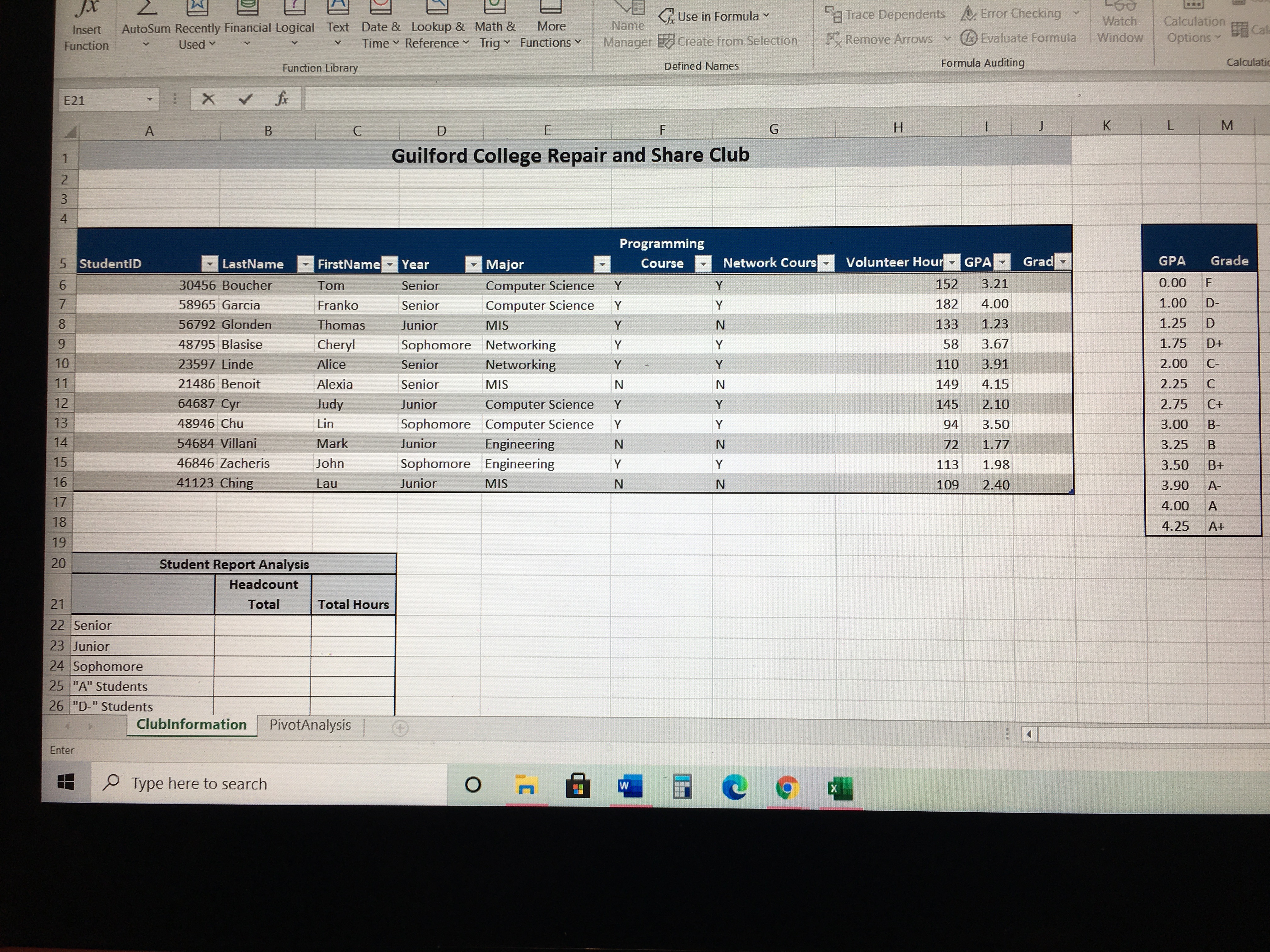
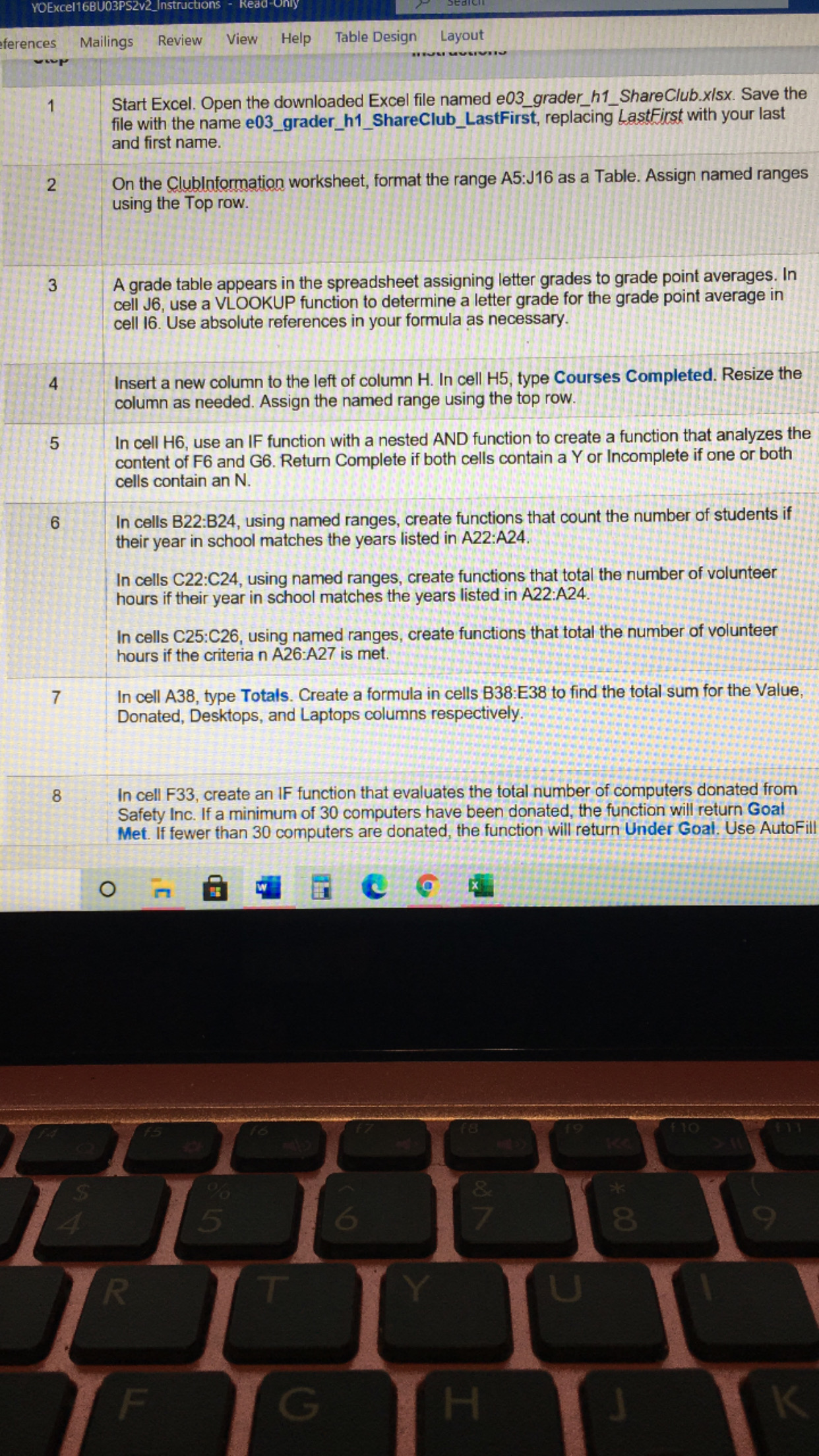
-60 " Use in Formula "Trace Dependents Error Checking Watch Calculation Name Insert AutoSum Recently Financial Logical Text Date & Lookup & Math & More Be Ca V Fx Remove Arrows & Evaluate Formula Window Options Manager Create from Selection Function Used Time ~ Reference ~ Trig Functions Calculati Function Library Defined Names Formula Auditing E21 X V G H K L M B C D Guilford College Repair and Share Club IN 4 Programming GPA 5 StudentID LastName . FirstName. Year Major Course . Network Cours " Volunteer Hour" GPA " Grad Grade 30456 Boucher Tom Senior Computer Science 152 3.21 0.00 F Y 182 4.00 1.00 D- 58965 Garcia Franko Senior Computer Science 1.25 8 56792 Glonden Thomas Junior MIS N 133 1.23 9 48795 Blasise Cheryl Sophomore Networking Y 58 3.67 1.75 D+ 2.00 C- 10 23597 Linde Alice Senior Networking Y 110 3.91 N 4.15 2.25 C Senior 149 11 21486 Benoit Alexia MIS 2.75 C+ 12 64687 Cyr Judy Junior Computer Science 145 2.10 Y 94 3.50 3.00 B- 13 48946 Chu Lin Sophomore Computer Science 14 54684 Villani Mark Junior Engineering N N 72 1.77 3.25 15 46846 Zacheris John Sophomore Engineering Y 113 1.98 3.50 B+ 16 41123 Ching Lau Junior MIS N N 109 2.40 3.90 A- 4.00 A 17 4.25 At 18 19 20 Student Report Analysis Headcount 21 Total Total Hours 22 Senior 23 Junior 24 Sophomore 25 "A" Students 26 "D-" Students Clubinformation PivotAnalysis Enter Type here to searchYOExcel16BU03PS2v2_Instructions ferences Mailings Review View Help Table Design Layout Start Excel. Open the downloaded Excel file named e03_grader_h1_ShareClub.xisx. Save the file with the name e03_grader_h1_ShareClub_LastFirst, replacing LastFirst with your last and first name. 2 On the Clubinformation worksheet, format the range A5:J16 as a Table. Assign named ranges using the Top row. 3 A grade table appears in the spreadsheet assigning letter grades to grade point averages. In cell J6, use a VLOOKUP function to determine a letter grade for the grade point average in cell 16. Use absolute references in your formula as necessary. Insert a new column to the left of column H. In cell H5, type Courses Completed. Resize the column as needed. Assign the named range using the top row. 5 In cell H6, use an IF function with a nested AND function to create a function that analyzes the content of F6 and G6. Return Complete if both cells contain a Y or Incomplete if one or both cells contain an N. 6 In cells B22:B24, using named ranges, create functions that count the number of students if their year in school matches the years listed in A22:A24. In cells C22:C24, using named ranges, create functions that total the number of volunteer hours if their year in school matches the years listed in A22:A24. In cells C25:C26, using named ranges, create functions that total the number of volunteer hours if the criteria n A26:A27 is met. N In cell A38, type Totals. Create a formula in cells B38:E38 to find the total sum for the Value, Donated, Desktops, and Laptops columns respectively. 8 In cell F33, create an IF function that evaluates the total number of computers donated from Safety Inc. If a minimum of 30 computers have been donated, the function will return Goal Met. If fewer than 30 computers are donated, the function will return Under Goal. Use AutoFi O & 5 8 9 R T Y U F G H K