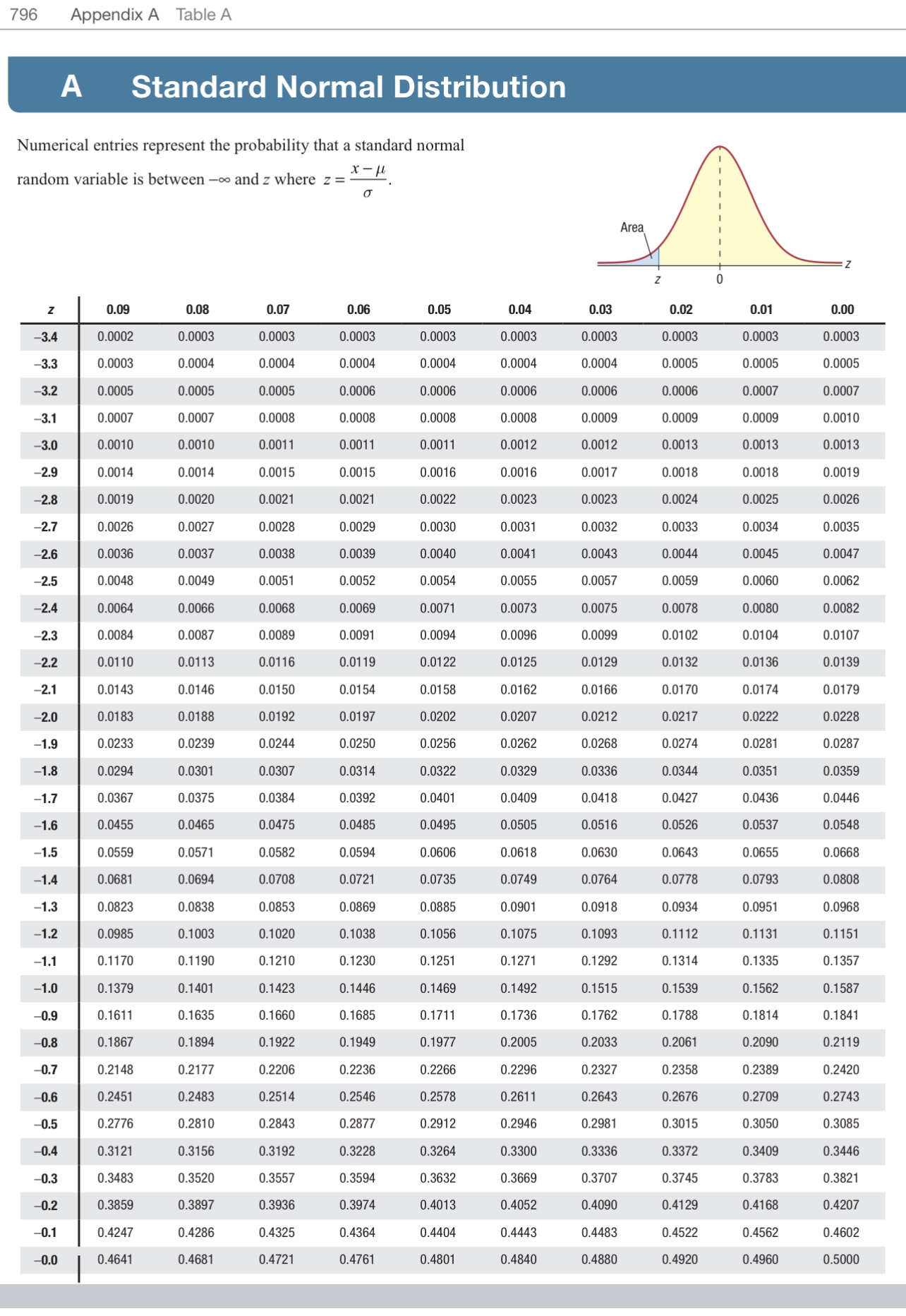
Question: 796 Appendix A Table A A Standard Normal Distribution Numerical entries represent the probability that a standard normal I random variable is between oo and

796 Appendix A Table A A Standard Normal796 Appendix A Table A A Standard Normal796 Appendix A Table A A Standard Normal796 Appendix A Table A A Standard Normal796 Appendix A Table A A Standard Normal796 Appendix A Table A A Standard Normal
796 Appendix A Table A A Standard Normal Distribution Numerical entries represent the probability that a standard normal I random variable is between oo and z where z = x _ #l l a 1 Area 5 I z z 0 Z 013 0.08 0.07 0.06 0.05 0.04 0.03 0.02 0.01 0.00 3.4 0.0002 0.01113 0.0003 0.0003 0.0003 0.0003 0.0003 0.0003 0.0003 0.0003 3.3 0.0003 0.0034 0.0004 0.0004 0.0004 0.0004 0.0004 0.0005 0.0005 0.0005 -3.2 0.0005 0.01115 0.0005 0.0006 0.0006 0.0008 0.0006 0.00% 0.0007 0.0007 3.1 0.0007 0.0007 0.0008 0.0008 0.0008 0.0008 0.0009 0.0009 0.0009 0.0010 -3.0 0.0010 0.0010 0.0011 0.0011 0.0011 0.0012 0.0012 0.0013 0.0013 0.0013 2.9 0.0014 0.0014 0.0015 0.0015 0.0016 0.0016 0.0017 0.0018 0.0018 0.0019 2.8 0.0019 0.0020 0.0021 0.0021 0.0022 0.0023 0.0023 0.0024 0.0025 0.0026 2.7 0.0026 0.0027 0.0028 0.0029 0.0030 0.0031 0.0032 0.0033 0.0034 0.0035 2.6 0.0036 0.0037 0.0038 0.0039 0.0040 0.0041 0.0043 0.0044 0.0045 0.0047 2.5 0.0040 0.0049 0.0051 0.0052 0.0054 0.0055 0.0057 0.0059 0.0060 0.0062 2.4 0.0064 mm 0.0068 0.0069 0.0071 0.0073 0.0075 0.0076 0.0080 0.0062 2.3 0.0084 0.0087 0.0089 0.0091 0.0094 0.0096 0.0099 0.0102 0.0104 0.0107 -2.2 0.0110 0.0113 0.0116 0.0119 0.0122 0.0125 0.0129 0.0132 0.0136 0.0139 2.1 0.0143 0.0146 0.0150 0.0154 0.0158 0.0162 0.0166 0.0170 0.0174 0.0179 2.0 0.0183 0.0168 0.0192 0.0197 0.0202 0.0207 0.0212 0.0217 0.0222 0.0228 1.9 0.0233 0.0239 0.0244 0.0250 0.0256 0.0262 0.0268 0.0274 0.0281 0.0287 1.8 0.0294 0.0301 0.0307 0.0314 0.0322 0.0329 0.0336 0.0044 0.0351 0.0359 1.7 0.0367 0.0375 0.0384 0.0392 0.0401 0.0409 0.041 8 0.0427 0.0436 0.0446 1.8 0.0455 0.0465 0.0475 0.0485 0.0495 0.0505 0.0516 0.0526 0.0537 0.0548 1.5 0.0559 0.0571 0.0582 0.0594 0.0606 0.0618 0.0630 0.0643 0.0655 0.0668 -1.4 0.0681 0.0694 0.0708 0.0721 0.07 35 0.0749 0.0764 0.0776 0.0793 0.0608 1.3 0.0823 0.0838 0.0853 0.0869 0.0885 0.0901 0.0918 0.0934 0.0951 0.0968 1.2 0.0985 0.11113 0.1020 0.1038 0.1056 0.1075 0.1093 0.1112 0.1131 0.1151 1.1 0.1170 0.1190 0.1210 0.1230 0.1251 0.1271 0.1292 0.1314 0.1335 0.1357 1.0 0.1379 0.1401 0.1423 0.1446 0.1469 0.1492 0.1515 0.1539 0.1562 0.1587 0.9 0.1611 0.1635 0.1660 0.1685 0.1711 0.1736 0.1762 0.1788 0.1814 0.1641 0.8 0.1867 0.1894 0.1922 0.1949 0.1977 0.2005 0.2033 0.2061 0.2090 0.2119 -0.7 0.2148 0.2177 0.2 206 0.2236 0.2266 0.2296 0.2327 0.2358 0.2389 0.2420 -0.6 0.2451 0.2483 0.2514 0.2546 0.2578 0.261 1 0.2643 0.2676 0.2709 0.2743 0.5 0.2776 0.2810 0.2 843 0.2877 0.2912 0.2946 0.2981 0.3015 0.3050 0.3085 41.4 0.3121 0.3156 0.3192 0.3228 0.3264 0.3300 0.3336 0.3372 0.3409 0.3446 0.3 0.3483 0.3520 0.3557 0.3594 0.36 32 0.3669 0.3707 0.3745 0.3783 0.3821 0.2 0.3859 0.3897 0.3936 0.3974 0.4013 0.4052 0.4090 0.4129 0.4166 0.4207 0.1 0.4247 0.4286 0.4325 0.4364 0.4404 0.4443 0.4483 0.4522 0.4562 0.4602 0.0 0.4641 0.4661 0.4721 0.4761 0.4801 0.4840 0.4860 0.4920 0.4960 0.5000 Appendix A Table B B Standard Normal Distribution Numerical entries represent the probability that a standard normal random variable is between -o and z where z = - x - H Area 0 Z 0.03 0.04 0.05 0.06 0.07 0.08 0.09 Z 0.00 0.01 0.02 0.0 0.5000 0.5040 0.5080 0.5120 0.5160 0.5199 0.5239 0.5279 0.5319 .5359 0.1 0.5398 0.5438 0.5478 0.5517 0.5557 0.5596 0.5636 0.5675 0.5714 0.5753 0.2 0.5832 0.5871 0.5910 0.5948 0.5987 0.6026 0.6064 0.6103 0.6141 0.5793 0.3 0.6179 0.6217 0.6255 0.6293 0.6331 0.6368 0.6406 0.6443 0.6480 0.6517 0.6844 0.6879 0.4 0.6554 0.6591 0.6628 0.6664 0.6700 0.6736 0.6772 0.6808 0.6915 0.6950 0.6985 0.7019 0.7054 0.7088 0.7123 0.7157 0.7190 0.7224 0.5 0.6 0.7257 0.7291 0.7324 0.7357 0.7389 0.7422 0.7454 0.7486 0.7517 0.7549 0.7 0.7580 0.7611 0.7642 0.7673 0.7704 0.7734 0.7764 0.7794 0.7823 0.7852 0.7881 0.7910 0.7939 0.7967 0.7995 0.8023 0.8051 0.8078 0.8106 0.8133 0.8 0.9 0.8389 0.8159 0.8186 0.8212 0.8238 0.8264 0.8289 0.8315 0.8340 0.8365 1.0 0.8413 0.8438 0.8461 0.8485 0.8508 0.8531 0.8554 0.8577 0.8599 0.8621 1.1 0.8643 0.8665 0.8686 0.8708 0.8729 0.8749 0.8770 0.8790 0.8810 0.8830 1 .2 0.8849 0.8869 0.8888 0.8907 0.8925 0.8944 0.8962 0.8980 0.8997 0.9015 1.3 0.9032 0.9049 0.9066 0.9082 0.9099 0.9115 0.9131 0.9147 0.9162 0.9177 1.4 0.9192 0.9207 0.9222 0.9236 0.9251 0.9265 0.9279 0.9292 0.9306 0.9319 0.9429 0.9441 1.5 0.9332 0.9345 0.9357 0.9370 0.9382 0.9394 0.9406 0.9418 1 . 6 0.9452 0.9463 0.9474 0.9484 0.9495 0.9505 0.9515 0.9525 0.9535 0.9545 0.9564 0.9573 0.9582 L696 0 0.9599 0.9608 0.9616 0.9625 0.9633 1.7 0.9554 1.8 0.9641 0.9649 0.9656 0.9664 0.9671 0.9678 0.9686 0.9693 0.9699 0.9706 1.9 0.9713 0.9719 0.9726 0.9732 0.9738 0.9744 0.9750 0.9756 0.9761 0.9767 2.0 0.9772 0.9778 0.9783 0.9788 0.9793 0.9798 0.9803 0.9808 0.9812 0.9817 0.9826 0.9830 0.9834 0.9838 0.9842 0.9846 0.9850 0.9854 0.9857 2.1 0.9821 2.2 0.9861 0.9864 0.9868 0.9871 0.9875 0.9878 0.9881 0.9884 0.9887 0.9890 2.3 0.9893 0.9896 0.9898 0.9901 0.9904 0.9906 0.9909 0.9911 0.9913 0.9916 2.4 0.9918 0.9920 0.9922 0.9925 0.9927 0.9929 0.9931 0.9932 0.9934 0.9936 2.5 0.9938 0.9940 0.9941 0.9943 0.9945 0.9946 0.9948 0.9949 0.9951 0.9952 2.6 0.9953 0.9955 0.9956 0.9957 0.9959 0.9960 0.9961 0.9962 0.9963 0.9964 2.7 0.9965 0.9966 0.9967 0.9968 0.9969 0.9970 0.9971 0.9972 0.9973 0.9974 2 .8 0.9974 0.9975 0.9976 0.9977 0.9977 0.9978 0.9979 0.9979 0.9980 0.9981 0.9982 0.9982 0.9983 0.9984 0.9984 0.9985 0.9985 0.9986 0.9986 2. 0.9981 3.0 0.9987 0.9987 0.9987 0.9988 0.9988 0.9989 0.9989 0.9989 0.9990 0.9990 3.1 0.9990 0.9991 0.9991 0.9991 0.9992 0.9992 0.9992 0.9992 0.9993 0.9993 3.2 0.9993 0.9993 0.9994 0.9994 0.9994 0.9994 0.9994 0.9995 0.9995 0.9995 3.3 0.9995 0.9995 0.9995 0.9996 0.9996 0.9996 0.9996 0.9996 0.9996 0.9997 3. 0.9997 0.9997 0.9997 0.9997 0.9997 0.9997 0.9997 0.9997 0.9997 0.9998Normal Distribution Activity: Setting the Curve Name: Date: Setting the Curve Dr. Groppe, a professor in the School of Computing at Klaggen University. is using a standardized nal exam that is "nationally normed\" for his Computer Science || class. Nationally normed implies that the normal distribution is an appropriate approximation for the probability distribution of students' scores on the exam. The probability distribution of students' scores on this standardized exam can be estimated using the normal distribution shown below. Note: An inection point is a calculus term that indicates a point on a curve where the curve changes from curving up to curving down or vice versa. The distance along the xaxis from one inection point to the mean is equal to the value of the standard deviation of the particular normal distribution. 1. State the mean of the distribution of the computer science exam scores based on the gure above. 2. State the standard deviation of the computer science exam scores based on the gure above. At some point in our academic pursuit, we all think that we would like our professors to curve our grades. Especially if we're the ones setting the curve. After considering his students' request to curve the grades on the nal exam, Dr. Groppe has come up with two options to use if he decides to curve the grades. Follow the steps listed to determine the grading scale for each option. Curved Grading Option #1 ' Students whose raw scores are at or above the 90'\" percentile will receive an A. ' Students whose raw scores are in the Both-89th percentile will receive a B. ' Students whose raw scores are in the Tom79'\" percentile will receive a C. ' Students whose raw scores are in the BOW69'" percentile will receive a D. ' Students whose raw scores are below the 60'h percentile will receive an F. 2 Normal Distribution Activity: Setting the Curve 3. In order to know the cutoff exam scores required for Curved Grading Option #1, Dr. Groppe needs to know what z-soores correspond to the upper limit percentiles. Find each z-score that corresponds to the following percentiles by using the cumulative normal distribution tables. Use the z-score with the percentage closest to the percentile. Round your z-scores to 2 decimal places. We've found the z-score of the 90"1 percentile for you. 90'\" percentile 1.28 80'\" percentile 70\"1 percentile 60th percentile 4. Using the z-scores found in Step 3, find the exam scores that correspond to Curved Grading Option #1. Assume that the exam scores range from 0 to 100. (Round to the nearest whole number.) Hint: You will need to use the z-score formula and solve for the data value. Curved Grading Option #1 A: - 100 B: Curved Grading Option #2 The second option for curving the grades is as follows: Students whose raw scores are at least two standard deviations above the mean of the standardized test will receive an A. - Students whose raw scores are from one up to two standard deviations above the mean of the standardized test will receive a B. - Students whose raw scores are from one standard deviation below the mean up to one standard deviation above the mean of the standardized test will receive a C. Students whose raw scores are from two standard deviations below the mean up to one standard deviation below the mean of the standardized test will receive a D. - Students whose raw scores are more than two standard deviations below the mean of the standardized test will receive an F. Normal Distribution Activity: Setting the Curve 3 5. Using the information above, find the exam scores that correspond to Curved Grading Option #2. Assume that the exam scores range from 0 to 100. (Round to the nearest whole number.) Curved Grading Option #2 Computer Science II Raw Exam Scores A: 100 Raw Score/ Name Uncurved Grade B J. Alexander 79/C C W. Thouy 69/D C. Bradford 88/B D: S. Nance 66/D A. Moore 75/C F: 0 K. Pinkston 86/B C. Navas 91/A R. Alexandru 77/C S. Garcia 82/B A partial list of raw scores for students in Dr. Groppe's Computer Science II class. 6. Using the grading scales you just created in Steps 4 and 5, complete the following table of the partial list of grades and find the new curved letter grades that the students would receive in each of the curving options given their raw scores on the exam. Computer Science II Final Exam Scores Raw Score/ Name Uncurved Grade Option #1 Curved Grade Option #2 Curved Grade J. Alexander 79/C W. Thouy 69/D C. Bradford 88/B S. Nance 66/D A. Moore 75/C K. Pinkston 86/B C. Navas 91/A R. Alexandru 77/C S. Garcia 82/B4 Normal Distribution Activity: Setting the Curve After reviewing the grades for each student using the two optional curving methods, answer the following questions. 7. Who do you think benefits the most from Curved Grading Option #1? Why? 8. Who is likely to disapprove of Curved Grading Option #1? Why? 9. Who do you think benefits the most from Curved Grading Option #2? Why? 10. Who is likely to disapprove of Curved Grading Option #2? Why? 11. Which grading scale do you feel is most fair? Explain why

Step by Step Solution

There are 3 Steps involved in it

1 Expert Approved Answer
Step: 1 Unlock blur-text-image
Question Has Been Solved by an Expert!

Get step-by-step solutions from verified subject matter experts

Step: 2 Unlock
Step: 3 Unlock

Students Have Also Explored These Related Mathematics Questions!