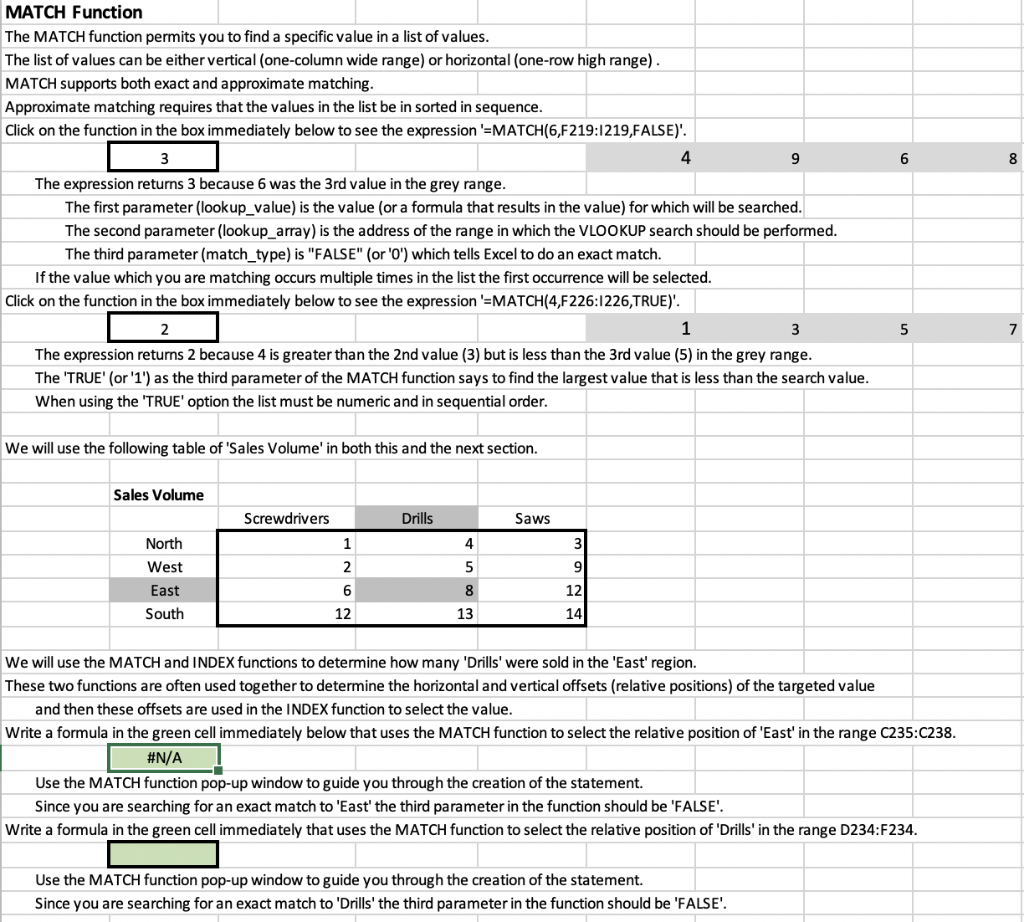
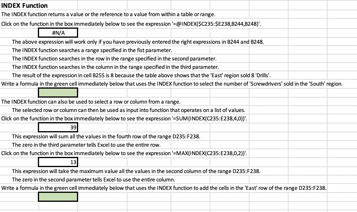
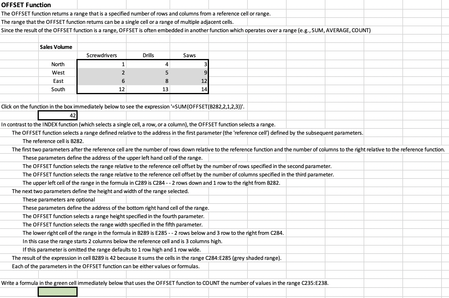
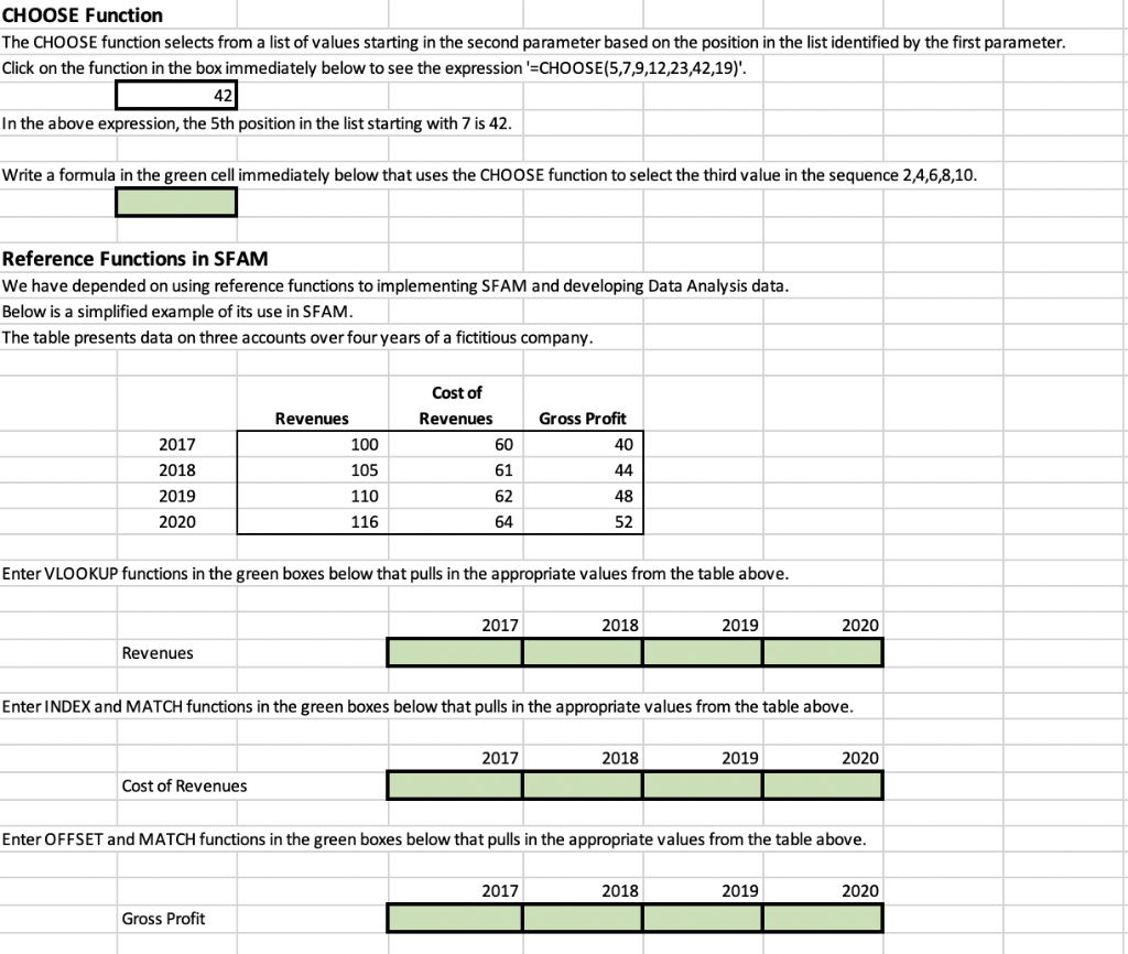
9 6 8 MATCH Function The MATCH function permits you to find a specific value in a list of values. The list of values can be either vertical (one-column wide range) or horizontal (one-row high range). MATCH supports both exact and approximate matching. Approximate matching requires that the values in the list be in sorted in sequence. Click on the function in the box immediately below to see the expression '=MATCH(6,F219:1219,FALSE)'. 3 4 The expression returns 3 because 6 was the 3rd value in the grey range. The first parameter (lookup_value) is the value (or a formula that results in the value) for which will be searched. The second parameter (lookup_array) is the address of the range in which the VLOOKUP search should be performed. The third parameter (match_type) is "FALSE" (or 'O') which tells Excel to do an exact match. If the value which you are matching occurs multiple times in the list the first occurrence will be selected. Click on the function in the box immediately below to see the expression '=MATCH(4,F226:1226,TRUE)'. 2 1 3 The expression returns 2 because 4 is greater than the 2nd value (3) but is less than the 3rd value (5) in the grey range. The 'TRUE' (or '1') as the third parameter of the MATCH function says to find the largest value that is less than the search value. When using the 'TRUE' option the list must be numeric and in sequential order. 5 7 We will use the following table of Sales Volume' in both this and the next section. Sales Volume Screwdrivers Drills Saws 1 4 3 2 5 9 North West East South 6 8 12 14 12 13 We will use the MATCH and INDEX functions to determine how many 'Drills' were sold in the 'East' region. These two functions are often used together to determine the horizontal and vertical offsets (relative positions) of the targeted value and then these offsets are used in the INDEX function to select the value. Write a formula in the green cell immediately below that uses the MATCH function to select the relative position of 'East' in the range C235:C238. #N/A Use the MATCH function pop-up window to guide you through the creation of the statement. Since you are searching for an exact match to 'East' the third parameter in the function should be 'FALSE'. Write a formula in the green cell immediately that uses the MATCH function to select the relative position of 'Drills' in the range D234:F234. Use the MATCH function pop-up window to guide you through the creation of the statement. Since you are searching for an exact match to 'Drills' the third parameter in the function should be 'FALSE'. INDEX Function The INDEX function returns a value or the reference to a value from within a table or range. Click on the function in the box immediately below to see the expression '=@INDEX($C235:$E238,B244,8248)'. #N/A The above expression will work only if you have previously entered the right expressions in B244 and B248. The INDEX function searches a range specified in the fist parameter. The INDEX function searches in the row in the range specified in the second parameter. The INDEX function searches in the column in the range specified in the third parameter. The result of the expression in cell B255 is 8 because the table above shows that the 'East' region sold 8 'Drills'. Write a formula in the green cell immediately below that uses the INDEX function to select the number of 'Screwdrivers' sold in the 'South' region. The INDEX function can also be used to select a row or column from a range. The selected row or column can then be used as input into function that operates on a list of values. Click on the function in the box immediately below to see the expression '=SUM(INDEX(C235:E238,4,0))'. 39 This expression will sum all the values in the fourth row of the range D235:F238. The zero in the third parameter tells Excel to use the entire row. Click on the function in the box immediately below to see the expression '=MAX(INDEX(C235:E238,0,2))'. 13 This expression will take the maximum value all the values in the second column of the range D235:F238. The zero in the second parameter tells Excel to use the entire column. Write a formula in the green cell immediately below that uses the INDEX function to add the cells in the 'East' row of the range D235:F238. OFFSET Function The OFFSET function returns a range that is a specified number of rows and columns from a reference cell or range. The range that the OFFSET function returns can be a single cell or a range of multiple adjacent cells. Since the result of the OFFSET function is a range, OFFSET is often embedded in another function which operates over a range (e.g., SUM, AVERAGE, COUNT) Sales Volume Screwdrivers Drills Saws 1 4 3 2 5 9 North West East South 6 8 12 12 13 14 Click on the function in the box immediately below to see the expression '=SUM(OFFSET(B282,2,1,2,3))'. 42 In contrast to the INDEX function (which selects a single cell, a row, or a column), the OFFSET function selects a range. The OFFSET function selects a range defined relative to the address in the first parameter (the 'reference cell') defined by the subsequent parameters. The reference cell is B282. The first two parameters after the reference cell are the number of rows down relative to the reference function and the number of columns to the right relative to the reference function. These parameters define the address of the upper left hand cell of the range. The OFFSET function selects the range relative to the reference cell offset by the number of rows specified in the second parameter. The OFFSET function selects the range relative to the reference cell offset by the number of columns specified in the third parameter. The upper left cell of the range in the formula in C289 is C284 -- 2 rows down and 1 row to the right from B282. The next two parameters define the height and width of the range selected. These parameters are optional These parameters define the address of the bottom right hand cell of the range. The OFFSET function selects a range height specified in the fourth parameter. The OFFSET function selects the range width specified in the fifth parameter. The lower right cell of the range in the formula in B289 is E285 -- 2 rows below and 3 row to the right from C284. In this case the range starts 2 columns below the reference cell and is 3 columns high. If this parameter is omitted the range defaults to 1 row high and 1 row wide. The result of the expression in cell B289 is 42 because it sums the cells in the range C284:E285 (grey shaded range). Each of the parameters in the OFFSET function can be either values or formulas. Write a formula in the green cell immediately below that uses the OFFSET function to COUNT the number of values in the range C235:E238. CHOOSE Function The CHOOSE function selects from a list of values starting in the second parameter based on the position in the list identified by the first parameter. Click on the function in the box immediately below to see the expression '=CHOOSE(5,7,9,12,23,42,19)'. 42 In the above expression, the 5th position in the list starting with 7 is 42. Write a formula in the green cell immediately below that uses the CHOOSE function to select the third value in the sequence 2,4,6,8,10. Reference Functions in SFAM We have depended on using reference functions to implementing SFAM and developing Data Analysis data. Below is a simplified example of its use in SFAM. The table presents data on three accounts over four years of a fictitious company. Cost of Revenues Revenues Gross Profit 2017 100 60 40 61 44 2018 2019 2020 105 110 48 62 64 116 52 Enter VLOOKUP functions in the green boxes below that pulls in the appropriate values from the table above. 2017 2018 2019 2020 Revenues Enter INDEX and MATCH functions in the green boxes below that pulls in the appropriate values from the table above. 2017 2018 2019 2020 Cost of Revenues Enter OFFSET and MATCH functions in the green boxes below that pulls in the appropriate values from the table above. 2017 2018 2019 2020 Gross Profit 9 6 8 MATCH Function The MATCH function permits you to find a specific value in a list of values. The list of values can be either vertical (one-column wide range) or horizontal (one-row high range). MATCH supports both exact and approximate matching. Approximate matching requires that the values in the list be in sorted in sequence. Click on the function in the box immediately below to see the expression '=MATCH(6,F219:1219,FALSE)'. 3 4 The expression returns 3 because 6 was the 3rd value in the grey range. The first parameter (lookup_value) is the value (or a formula that results in the value) for which will be searched. The second parameter (lookup_array) is the address of the range in which the VLOOKUP search should be performed. The third parameter (match_type) is "FALSE" (or 'O') which tells Excel to do an exact match. If the value which you are matching occurs multiple times in the list the first occurrence will be selected. Click on the function in the box immediately below to see the expression '=MATCH(4,F226:1226,TRUE)'. 2 1 3 The expression returns 2 because 4 is greater than the 2nd value (3) but is less than the 3rd value (5) in the grey range. The 'TRUE' (or '1') as the third parameter of the MATCH function says to find the largest value that is less than the search value. When using the 'TRUE' option the list must be numeric and in sequential order. 5 7 We will use the following table of Sales Volume' in both this and the next section. Sales Volume Screwdrivers Drills Saws 1 4 3 2 5 9 North West East South 6 8 12 14 12 13 We will use the MATCH and INDEX functions to determine how many 'Drills' were sold in the 'East' region. These two functions are often used together to determine the horizontal and vertical offsets (relative positions) of the targeted value and then these offsets are used in the INDEX function to select the value. Write a formula in the green cell immediately below that uses the MATCH function to select the relative position of 'East' in the range C235:C238. #N/A Use the MATCH function pop-up window to guide you through the creation of the statement. Since you are searching for an exact match to 'East' the third parameter in the function should be 'FALSE'. Write a formula in the green cell immediately that uses the MATCH function to select the relative position of 'Drills' in the range D234:F234. Use the MATCH function pop-up window to guide you through the creation of the statement. Since you are searching for an exact match to 'Drills' the third parameter in the function should be 'FALSE'. INDEX Function The INDEX function returns a value or the reference to a value from within a table or range. Click on the function in the box immediately below to see the expression '=@INDEX($C235:$E238,B244,8248)'. #N/A The above expression will work only if you have previously entered the right expressions in B244 and B248. The INDEX function searches a range specified in the fist parameter. The INDEX function searches in the row in the range specified in the second parameter. The INDEX function searches in the column in the range specified in the third parameter. The result of the expression in cell B255 is 8 because the table above shows that the 'East' region sold 8 'Drills'. Write a formula in the green cell immediately below that uses the INDEX function to select the number of 'Screwdrivers' sold in the 'South' region. The INDEX function can also be used to select a row or column from a range. The selected row or column can then be used as input into function that operates on a list of values. Click on the function in the box immediately below to see the expression '=SUM(INDEX(C235:E238,4,0))'. 39 This expression will sum all the values in the fourth row of the range D235:F238. The zero in the third parameter tells Excel to use the entire row. Click on the function in the box immediately below to see the expression '=MAX(INDEX(C235:E238,0,2))'. 13 This expression will take the maximum value all the values in the second column of the range D235:F238. The zero in the second parameter tells Excel to use the entire column. Write a formula in the green cell immediately below that uses the INDEX function to add the cells in the 'East' row of the range D235:F238. OFFSET Function The OFFSET function returns a range that is a specified number of rows and columns from a reference cell or range. The range that the OFFSET function returns can be a single cell or a range of multiple adjacent cells. Since the result of the OFFSET function is a range, OFFSET is often embedded in another function which operates over a range (e.g., SUM, AVERAGE, COUNT) Sales Volume Screwdrivers Drills Saws 1 4 3 2 5 9 North West East South 6 8 12 12 13 14 Click on the function in the box immediately below to see the expression '=SUM(OFFSET(B282,2,1,2,3))'. 42 In contrast to the INDEX function (which selects a single cell, a row, or a column), the OFFSET function selects a range. The OFFSET function selects a range defined relative to the address in the first parameter (the 'reference cell') defined by the subsequent parameters. The reference cell is B282. The first two parameters after the reference cell are the number of rows down relative to the reference function and the number of columns to the right relative to the reference function. These parameters define the address of the upper left hand cell of the range. The OFFSET function selects the range relative to the reference cell offset by the number of rows specified in the second parameter. The OFFSET function selects the range relative to the reference cell offset by the number of columns specified in the third parameter. The upper left cell of the range in the formula in C289 is C284 -- 2 rows down and 1 row to the right from B282. The next two parameters define the height and width of the range selected. These parameters are optional These parameters define the address of the bottom right hand cell of the range. The OFFSET function selects a range height specified in the fourth parameter. The OFFSET function selects the range width specified in the fifth parameter. The lower right cell of the range in the formula in B289 is E285 -- 2 rows below and 3 row to the right from C284. In this case the range starts 2 columns below the reference cell and is 3 columns high. If this parameter is omitted the range defaults to 1 row high and 1 row wide. The result of the expression in cell B289 is 42 because it sums the cells in the range C284:E285 (grey shaded range). Each of the parameters in the OFFSET function can be either values or formulas. Write a formula in the green cell immediately below that uses the OFFSET function to COUNT the number of values in the range C235:E238. CHOOSE Function The CHOOSE function selects from a list of values starting in the second parameter based on the position in the list identified by the first parameter. Click on the function in the box immediately below to see the expression '=CHOOSE(5,7,9,12,23,42,19)'. 42 In the above expression, the 5th position in the list starting with 7 is 42. Write a formula in the green cell immediately below that uses the CHOOSE function to select the third value in the sequence 2,4,6,8,10. Reference Functions in SFAM We have depended on using reference functions to implementing SFAM and developing Data Analysis data. Below is a simplified example of its use in SFAM. The table presents data on three accounts over four years of a fictitious company. Cost of Revenues Revenues Gross Profit 2017 100 60 40 61 44 2018 2019 2020 105 110 48 62 64 116 52 Enter VLOOKUP functions in the green boxes below that pulls in the appropriate values from the table above. 2017 2018 2019 2020 Revenues Enter INDEX and MATCH functions in the green boxes below that pulls in the appropriate values from the table above. 2017 2018 2019 2020 Cost of Revenues Enter OFFSET and MATCH functions in the green boxes below that pulls in the appropriate values from the table above. 2017 2018 2019 2020 Gross Profit