

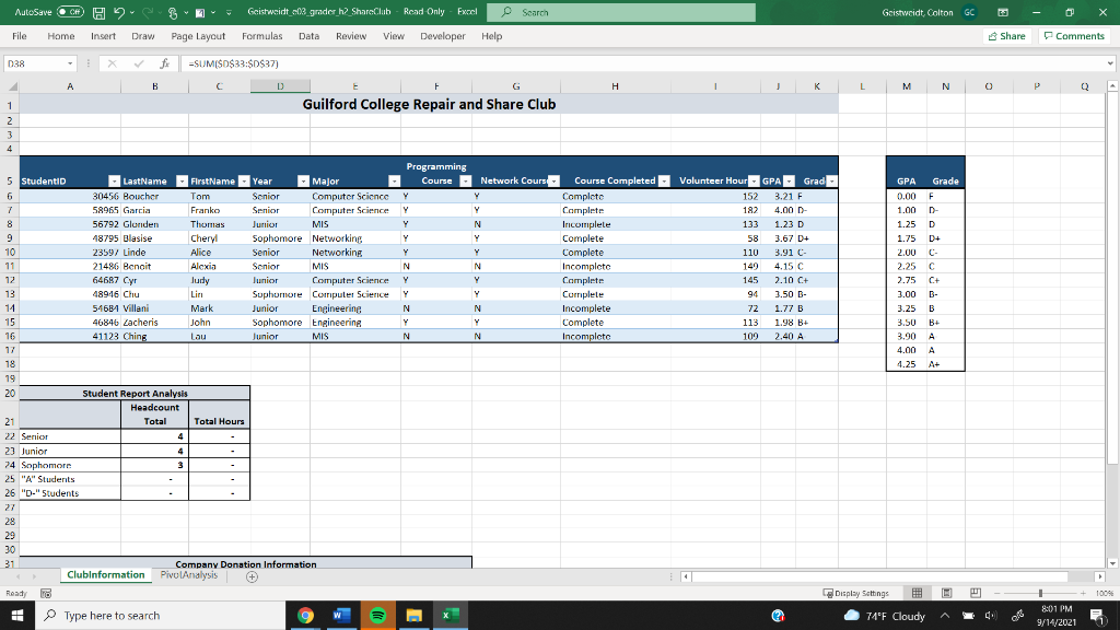
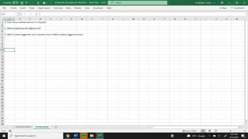
Question: 9 Using the data in the table, insert a PivotTable in cell A10 on the PivotAnalysis worksheet. Use the following criteria to create the PivotTable:
| 9 | Using the data in the table, insert a PivotTable in cell A10 on the PivotAnalysis worksheet. Use the following criteria to create the PivotTable: Add the Major and GPA fields to the FILTERS area (in that order). Add the Grade, Year, and FirstName fields to the ROWS area (in that order). Add the Volunteer Hours and LastName fields to the VALUES area (in that order). Display subtotals at the bottom of each group. In cell A10, type Grades. In cell B10, type Total Hours. In cell C10, type Total Students. Resize the columns as needed. |
| 10 | Insert a slicer for the Grade field. Format the slicer with 3 columns. Resize the slicer to remove the extra white space at the bottom. Move the slicer so the top-left corner is in cell F10. |
| 11 | In the slicer, select A, A-, B+, and B-. View the PivotTable data to determine how many students have a grade of an A or a B. Click cell A2, click the drop-down arrow, and then select the number of students. |
| 12 | Clear the filter in the slicer, and then in the slicer select the grade of an A. In cell B8, filter the data so the student with the highest GPA displays. View the PivotTable data to determine which student has the highest GPA. Click cell A4, click the drop-down arrow, and the select the name of the student with the highest GPA displayed. |
Step by Step Solution
There are 3 Steps involved in it

Get step-by-step solutions from verified subject matter experts