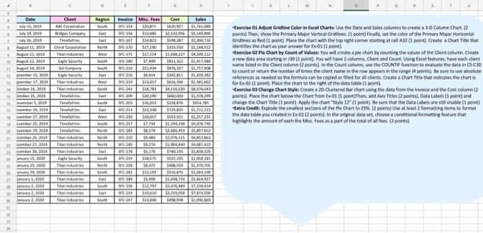
A 3 4 5 6 7 8 9 10 11 12 13 14 15 16 17 18 19 20 21 22 23 24 25 26 27 28 29 30 31 32 33 34 B Date July 15, 2019 July 19, 2019 July 26, 2019 August 11, 2019 August 15, 2019 August 22, 2019 August 24, 2019 ptember 15, 2019 ptember 17, 2019 October 16, 2019 October 25, 2019 ovember 5, 2019 ovember 19, 2019 ovember 27, 2019 ovember 25, 2019 ovember 29, 2019 ecember 25, 2019 ecember 27, 2019 ecember 30, 2019 anuary 15, 2020 anuary 25, 2020 anuary 29, 2020 January 1, 2020 January 2, 2020 January 2, 2020 January 2, 2020 C Client ABC Corporation Bridges Company Timefall Inc. Chiral Corporation Titan Industries Eagle Security Sol Company Eagle Security Titan Industries Titan Industries Timefall Inc. Timefall Inc. Timefall Inc. Timefall Inc. Timefall Inc. Timefall Inc. Titan Industries Titan Industries Titan Industries Eagle Security Titan Industries Titan Industries Titan Industries Titan Industries Titan Industries Titan Industries D Region South East East North West South South East West South East South East West South North North North East South North South East South East South E F H Invoice Misc. Fees Cost Sales SFC-154 $20,871 $620,927 $1,741,089 SFC-156 $13,685 $2,532,956 $5,149,890 SFC-167 $14,823 $598,287 $2,300,710 SFC-170 $17,190 $319,550 $1,148,912 SFC-175 $17,154 $1,698,227 $4,599,112 SFC-180 $7,499 $913,322 $1,917,080 SFC-210 $21,434 $876,327 $1,757,908 SFC-216 $6,914 $342,811 $1,209,282 SFC-219 $13,657 $616,396 $1,581,662 SFC-244 $18,783 $4,116,020 $8,376,043 SFC-209 $20,190 $660,000 $1,978,299 SFC-203 $16,053 $228,876 $914,785 SFC-213 $23,338 $729,835 $1,711,222 SFC-230 $10,057 $553,551 $1,257,231 SFC-237 $7,734 $1,244,348 $4,078,740 SFC-183 $8,574 $2,686,453 $5,897,652 SFC-210 $9,483 $2,076,115 SFC-240 $9,276 SFC-178 $5,176 SFC-219 $18,575 SFC-228 $8,472 $488,559 $1,370,705 SFC-182 $13,193 $516,876 $1,683,109 SFC-189 $5,099 $1,698,733 $5,664,927 SFC-196) $12,797 $2,476,489. $7,239,424 SFC-219 $19,610 $3,219,058 $7,874,500 SFC-247 $13,048 $498,938 $1,096,869 $4,852,863 $1,904,840 $4,687,422 $740,195 $1,838,220 $525,195 $1,958,181 J K L M N P Q R S T U Exercise 01 Adjust Gridline Color in Excel Charts: Use the Date and Sales columns to create a 3-D Column Chart. (2 points) Then, show the Primary Major Vertical Gridlines. (1 point) Finally, set the color of the Primary Major Horizontal Gridlines as Red (1 point). Place the chart with the top right corner starting at cell A32 (1 point). Create a Chart Title that identifies the chart as your answer for Ex-01 (1 point). Exercise 02 Pie Chart by Count of Values: You will create a pie chart by counting the values of the Client column. Create a new data area starting in J30 (1 point). You will have 2 columns, Client and Count. Using Excel features, have each client name listed in the Client column (2 points). In the Count column, use the COUNTIF function to evaluate the data in C5:C30 to count or return the number of times the client name in the row appears in the range (4 points). Be sure to use absolute references as needed so the formula can be copied or filled for all clients. Create a Chart Title that indicates the chart is for Ex-02 (1 point). Place the chart to the right of the data table (1 point). Exercise 03 Change Chart Style: Create a 2D Clustered Bar chart using the data from the Invoice and the Cost column (2 points). Place the chart below the Chart from Ex-01 (1 point)Then, add Axis Titles (2 points), Data Labels (1 point) and change the Chart Title (1 point). Apply the chart "Style 12" (1 point). Be sure that the Data Labels are still visable (1 point) *Extra Credit: Explode the smallest sections of the Pie Chart to 25%. (2 points) Use at least 2 formatting items to format the data table you created in Ex-02 (2 points). In the original data set, choose a conditional formatting feature that highlights the amount of each the Misc. Fees as a part of the total of all fees. (2 points)

-[xescise 01 Adurt Gridline Color in Excel Charte Use the Dase and Soles columns to create a 1-D Column Chart R points) Then, show the Primary Major Wertical Gndines. II point] Finsly, set the color of the Prrmary Major Horltontal Gidlines as Red (1 point). Place the chart with the top right corner startine at cell A32 (1 point). Create a Chart Trle that idecties the chart as vour amwer for fx-ot (1 point). -Exercise 02 Ple Chart by Count of Values: You wil create a pie chart by courcing the values of the Clent column. Create a new dat area starting in 130 (1 point). You wil have 2 columns, Client and Count. Using Excel features, have esch clent to count or reburn the number of times the client name in the roa appean in the rarge (4 pointsl be sure to use absolute references as needed so the formula can be cosicd or fled for al clienta. Create a Chart Title that indicates the chert is for 6 - 02 (1 poind. Face the chart to the riets of the data table it peint) change the Chart Trie (1 point). Apply the chart "Style 12" (I point) Be sure ther the Data iabeis are still vicable (1 point) the data table vav created in 6 - 02 (2 pointa), in the orignal data set, choose a condtional formatting feature that hichlights the amount of each the Msc. Fees as a part of the total of all foes. Q points) -[xescise 01 Adurt Gridline Color in Excel Charte Use the Dase and Soles columns to create a 1-D Column Chart R points) Then, show the Primary Major Wertical Gndines. II point] Finsly, set the color of the Prrmary Major Horltontal Gidlines as Red (1 point). Place the chart with the top right corner startine at cell A32 (1 point). Create a Chart Trle that idecties the chart as vour amwer for fx-ot (1 point). -Exercise 02 Ple Chart by Count of Values: You wil create a pie chart by courcing the values of the Clent column. Create a new dat area starting in 130 (1 point). You wil have 2 columns, Client and Count. Using Excel features, have esch clent to count or reburn the number of times the client name in the roa appean in the rarge (4 pointsl be sure to use absolute references as needed so the formula can be cosicd or fled for al clienta. Create a Chart Title that indicates the chert is for 6 - 02 (1 poind. Face the chart to the riets of the data table it peint) change the Chart Trie (1 point). Apply the chart "Style 12" (I point) Be sure ther the Data iabeis are still vicable (1 point) the data table vav created in 6 - 02 (2 pointa), in the orignal data set, choose a condtional formatting feature that hichlights the amount of each the Msc. Fees as a part of the total of all foes. Q points)