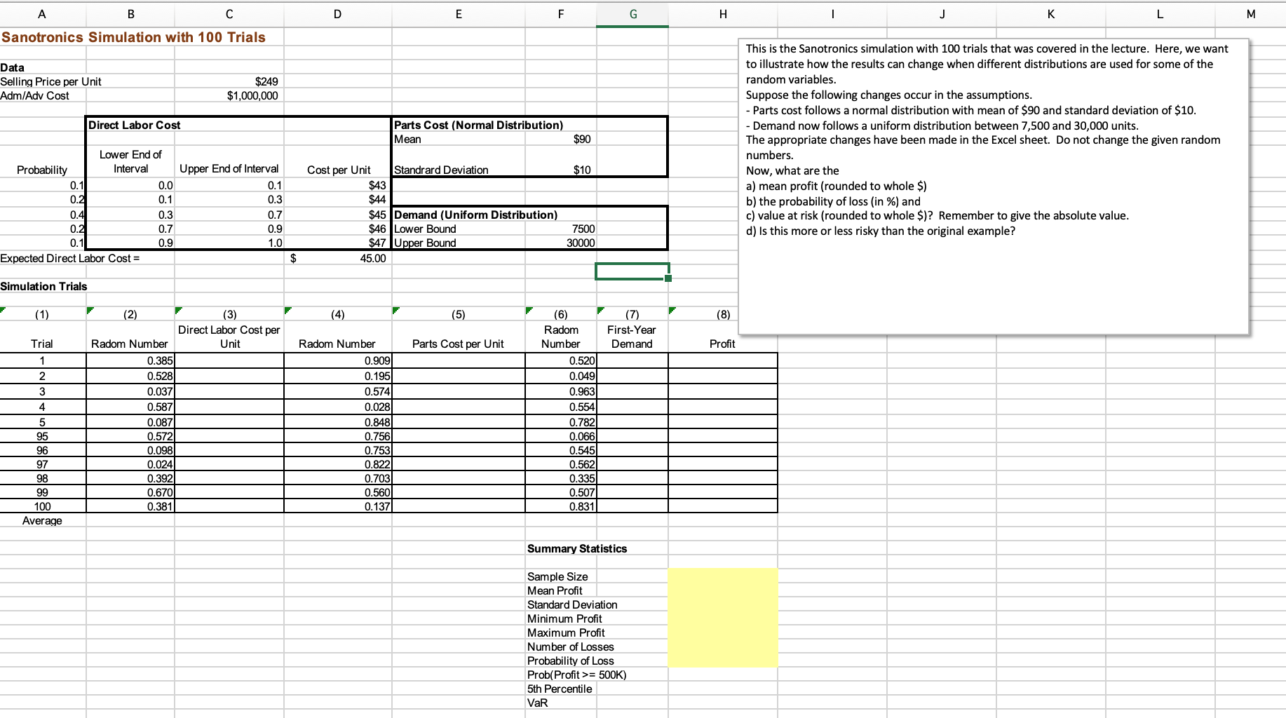
A B C D E F G . J K L M Sanotronics Simulation with 100 Trials Data Selling Price per Unit Adm/Adv Cost $249 $1,000,000 Direct Labor Cost Parts Cost (Normal Distribution) Mean $90 This is the Sanotronics simulation with 100 trials that was covered in the lecture. Here, we want to illustrate how the results can change when different distributions are used for some of the random variables. Suppose the following changes occur in the assumptions. - Parts cost follows a normal distribution with mean of $90 and standard deviation of $10. - Demand now follows a uniform distribution between 7,500 and 30,000 units. The appropriate changes have been made in the Excel sheet. Do not change the given random numbers. Now, what are the a) mean profit (rounded to whole $) b) the probability of loss (in %) and c) value at risk (rounded to whole $)? Remember to give the absolute value. d) Is this more or less risky than the original example? $10 Lower End of Probability Interval 0.1 0.0 0.2 0.1 0.4 0.3 0.2 0.7 0.1 0.9 Expected Direct Labor Cost = Upper End of Interval 0.1 0.3 0.7 0.9 1.0 Cost per Unit Standrard Deviation $43 $44 $45 Demand (Uniform Distribution) $46 Lower Bound $47 Upper Bound 45.00 7500 30000 $ Simulation Trials (1) (2) (4) (5) (8) (3) Direct Labor Cost per Unit First-Year Demand Trial Parts Cost per Unit Profit 1 2 3 4 5 95 96 97 98 99 100 Average Radom Number 0.385 0.528 0.037 0.587 0.087 0.572 0.098 0.024 0.392 0.670 0.381 Radom Number 0.909) 0.1951 0.574) 0.028 0.848) 0.756 0.753 0.822 0.7031 0.560 0.1371 (6) Radom Number 0.520 0.049 0.963 0.554 0.782 0.066 0.545 0.562 0.335 0.507 0.831 Summary Statistics Sample Size Mean Profit Standard Deviation Minimum Profit Maximum Profit Number of Losses Probability of Loss Prob(Profit >= 500K) 5th Percentile VaR A B C D E F G . J K L M Sanotronics Simulation with 100 Trials Data Selling Price per Unit Adm/Adv Cost $249 $1,000,000 Direct Labor Cost Parts Cost (Normal Distribution) Mean $90 This is the Sanotronics simulation with 100 trials that was covered in the lecture. Here, we want to illustrate how the results can change when different distributions are used for some of the random variables. Suppose the following changes occur in the assumptions. - Parts cost follows a normal distribution with mean of $90 and standard deviation of $10. - Demand now follows a uniform distribution between 7,500 and 30,000 units. The appropriate changes have been made in the Excel sheet. Do not change the given random numbers. Now, what are the a) mean profit (rounded to whole $) b) the probability of loss (in %) and c) value at risk (rounded to whole $)? Remember to give the absolute value. d) Is this more or less risky than the original example? $10 Lower End of Probability Interval 0.1 0.0 0.2 0.1 0.4 0.3 0.2 0.7 0.1 0.9 Expected Direct Labor Cost = Upper End of Interval 0.1 0.3 0.7 0.9 1.0 Cost per Unit Standrard Deviation $43 $44 $45 Demand (Uniform Distribution) $46 Lower Bound $47 Upper Bound 45.00 7500 30000 $ Simulation Trials (1) (2) (4) (5) (8) (3) Direct Labor Cost per Unit First-Year Demand Trial Parts Cost per Unit Profit 1 2 3 4 5 95 96 97 98 99 100 Average Radom Number 0.385 0.528 0.037 0.587 0.087 0.572 0.098 0.024 0.392 0.670 0.381 Radom Number 0.909) 0.1951 0.574) 0.028 0.848) 0.756 0.753 0.822 0.7031 0.560 0.1371 (6) Radom Number 0.520 0.049 0.963 0.554 0.782 0.066 0.545 0.562 0.335 0.507 0.831 Summary Statistics Sample Size Mean Profit Standard Deviation Minimum Profit Maximum Profit Number of Losses Probability of Loss Prob(Profit >= 500K) 5th Percentile VaR