

A brewery would like to study customer reception from male and female individuals to a new...
Fantastic news! We've Found the answer you've been seeking!
Question:


Transcribed Image Text:
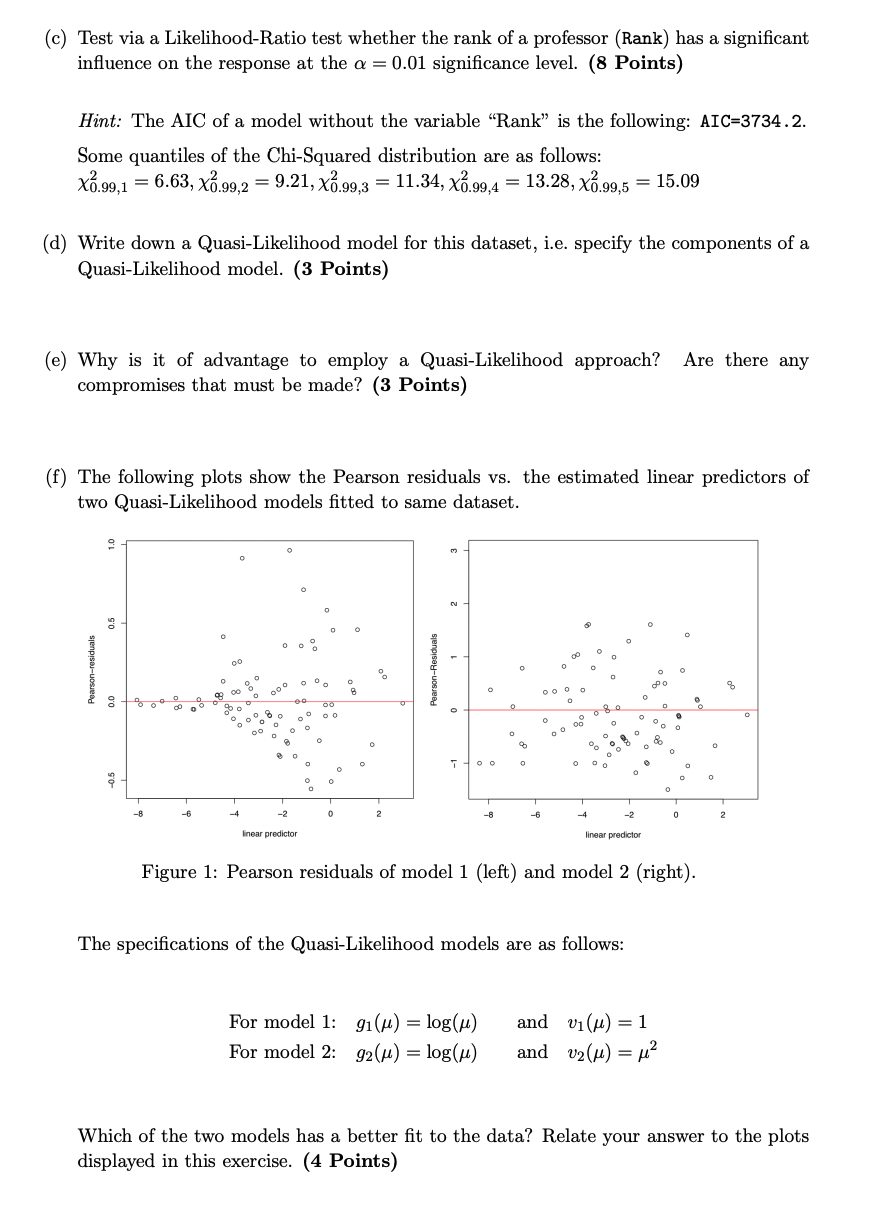
A brewery would like to study customer reception from male and female individuals to a new beer. They defined the customers' reaction to the beer as good (y = 1) and not good (y = 0), whereas also the covariate Gender is a dummy variable. This analysis should be carried out using a logit model with the following linear predictor: n = 30 + Gender 31, where the gender male is taken as reference category. a) Specify the logit model. Show that the Bernoulli distribution belongs to the exponential family of distributions. Write down the components: Ou di b(di), c(yi, i), as well as the link and response functions. Does the employed link function has any special properties? Additionally, write down the link function of the probit model. (6 Points) b) Derive the general form of the expected and observed Fisher information matrix for the logit model with intercept, a single covariate x, and independent observations (y, 2i), i = 1,..., n. (5 Points) c) A beer tasting session that consisted of n participants resulted in the following table: y=0|y=1 0.30 Gender = 0 0.29 Gender 1 0.24 0.17 Compute the maximum likelihood estimator for 30 and 3. Briefly interpret these coefficients. (7 Points) d) Would you be able to test whether the coefficients 30 and 3 are significantly different from zero using the data from exercise c)? (2 Points) Problem 2 Consider the dataset Salaries from the R package carData. The dataset contains the salaries (in 1000 USD) of n = 397 professors from the United States. A model with the following variables was fitted to the data: Variable Salary Gender TimeS YsP Disc Rank Coefficients: (Intercept) Gender TimeS YsP Disc = RankAssociate RankFull === Below is a snippet of the summary output of a model that contains all main effects: glm (formula Salary Gender + TimeS + YsP + Disc + Rank, family = gaussian (link = "log")) Description Salary in 1000 USD Gender Time spent in the current position Years since obtaining a PhD Discipline Rank or status of the professor Range Salary R+ Female (0) or male (1) TimeS No YSP No Estimate Std. Error t value 4.260286 0.049103 86.762 0.045782 0.036895 1.241 -0.003758 0.001675 -2.244 0.004292 0.001918 2.238 0.121638 0.149974 0.439736 theoretical (0) or applied (1) Assistant, Associate or Full Pr (>|t|) < 2e-16 *** 0.21539 0.02540 * 0.02581 * 0.020468 5.943 6.22e-09 *** 0.046593 3.219 0.00139 ** 0.043083 10.207 <2e-16 *** 27 Points Signif. codes: 0*** 0.001 '**' 0.01 '*' 0.05 . 0.1 '.' ' 1 I (Dispersion parameter for gaussian family taken to be 509.7898) Null deviance: 363301 on 396 degrees of freedom Residual deviance: 198817 on 390 degrees of freedom AIC: 3610.5 Number of Fisher Scoring iterations: 5 (a) Write down the structural assumption from this model, the linear predictor, as well as the distributional assumption (you don't need to write down all of the covariates). Make an assessment regarding the choices of the systematic and random components. Is the GLM fitted in the code able to model / capture any possible heteroscedasticity in the data? (5 Points) (b) Interpret the estimated coefficient of RankAssociate. Write down the formula used to estimate the dispersion parameter and interpret this parameter in context with the fitted model from above. (4 Points) (c) Test via a Likelihood-Ratio test whether the rank of a professor (Rank) has a significant influence on the response at the a = 0.01 significance level. (8 Points) Hint: The AIC of a model without the variable "Rank" is the following: AIC=3734.2. Some quantiles of the Chi-Squared distribution are as follows: X0.99,1 = = 6.63, x.99,2 = 9.21, x.99,3 = 11.34, X.99,4 13.28, X.99,5 = 15.09 (d) Write down a Quasi-Likelihood model for this dataset, i.e. specify the components of a Quasi-Likelihood model. (3 Points) (e) Why is it of advantage to employ a Quasi-Likelihood approach? Are there any compromises that must be made? (3 Points) (f) The following plots show the Pearson residuals vs. the estimated linear predictors of two Quasi-Likelihood models fitted to same dataset. 9 2 00 00 O 0 0 000 8 -2 linear predictor O O O 0 0 00 0 0 2 For model 1: For model 2: N T = O -8 91() = log() 92() = log() 0 D 0 8 0 -6 0 000 O no a 9 0 000 o -4 00 10 0 O a oc 8 C 0 -2 linear predictor The specifications of the Quasi-Likelihood models are as follows: 0 do 0 and v () = 1 and v() = 0 9 0 o T 0 Figure 1: Pearson residuals of model 1 (left) and model 2 (right). 0 o 0 0 0 2 8 O Which of the two models has a better fit to the data? Relate your answer to the plots displayed in this exercise. (4 Points) Problem 3 Assume that you have been given a metric response variable y; E R, a p-dimensional vector of covariates x, and that the i = 1,..., n observations are independent. The (n p) design matrix is denoted by X and it has been standardized, i.e. each column of X has a mean equal to 0 and variance equal to 1. (a) Derive the Ridge estimator R, i.e. the estimator that minimizes the following target function, where A is the penalty parameter: (5 Points) beta R (b) Consider the following plot of n = 100 simulated observations and p = 10 regression coefficients. The values of the estimated coefficients are displayed on the y-axis, whereas the x-axis shows values for A. Explain the basic idea behind the plot, including the path of the coefficients. Additionally, describe what happens in the extreme cases of X. (6 Points) 1.5 1.0 0.5 -1.0 -0.5 0.0 BR = arg min 3 ((y - XB) (y X) + \) - 0 100 17 Points lambda 200 300 (c) What are the differences between the penalty term of the Ridge estimator, the penalty term of the Penalized Least Squares estimator used for P-splines, and the penalty term of the Lasso estimator? Describe how the optimization with respect to finding an optimal penalty parameter could be carried out. (6 Points) Problem 4 A company wishes to analyse the satisfaction of n customers. The reponse variable Y has three values: Not satisfied (r = 1), satisfied (r = 2), very satisfied (r = 3). The covariates in the data are Gender and Age. The company wishes to carry out the analysis based on a cumulative Probit model. This model can be motivated using the latent variable U = -xy + where holds, and Y = r Or-1 < U Or. (a) Explain the idea behind the model by means of a sketch / illustration. (3 Points) (b) Write down the distribution of e, as well as the model equation for P(Y rx). Additionally, explain how P(Y = r|x) can be calculated. (3 Points) (c) How can the 0j, j = 1,..., k-1 be interpreted? (2 Points) - = 00 < 01 < < 0k-1 < 0k = (d) Explain briefly why a multinomial model should not be employed for this data. Mention one alternative to accomodate the presented type of response that also results in a categorical model for an ordinal response. Describe briefly the model class in general and write down the model equation. (4 Points) Consider now a categorical regression model fitted to the alligator dataset, which is known from the exercises of this course. The response variable is the Nourishment/ food of the alligators with response values: Fish, Invertebrata and Other. The covariates in the dataset were Gender (with male being reference category) and BodyLength (in cm). The covariate BodyLength has been centered for this analysis. The R output of the model is shown below: > summary (MultinomLogitModel) Call: multinom (formula = Nourishment Gender BodyLength) Coefficients: Fish Inver. Std. Errors: Fish Inver. (Intercept) GenderF BodyLength 0.158 1.365 19 Points 0.942 5.454 (Intercept) GenderF 1.197 0.783 1.849 0.924 0.087 -0.443 BodyLength 0.484 1.018 Page 5 of 9 (a) Compute the following odds: Odds of the response being Invertebrata relative to Other, for a male alligator of body size 10cm longer than the average. (2 Points) Odds of the response being Fish relative to the reference category, for a female alligator of average body length. (2 Points) (b) What is the nourishment/ food category with the highest odds for a male alligator with average body length? (3 Points) Problem 5 Consider a regression model of the form: Yi | Zi~ Exp(x), where the response is assumed to follow an Exponential distribution. component is specified as follows: m 14 - - - E[yi zi] fbi = = = exp |v;B;(z Xi B;(5=)). n Yi lp(y) = (-log(i) H) - 2 STK TKY, i=1 where it is assumed that is fixed. where B,..., Bm are suitable basis functions. The coefficients = (71,...,m) are estimated using a penalized Maximum-Likelihood approach, i.e. via maximization of the penalized log-likelihood (a) The penalty term is given by m 17 Points The systematic Ey Ky = ((v Vj-1) 2(Yj-1 Vj-2) + (Vj-2 Vj-3)). - - j=4 Derive the corresponding matrix of differences D and write down the penalty matrix K for the case of m= 6. What is the order d of differences used in this case? (6 Points) (b) Derive the score function of the penalized log-likelihood lp(y). (6 Points) (c) Describe (briefly) an iterative method / algorithm that is used to maximize the pe- nalised log-likelihood lp(y). (5 Points) A brewery would like to study customer reception from male and female individuals to a new beer. They defined the customers' reaction to the beer as good (y = 1) and not good (y = 0), whereas also the covariate Gender is a dummy variable. This analysis should be carried out using a logit model with the following linear predictor: n = 30 + Gender 31, where the gender male is taken as reference category. a) Specify the logit model. Show that the Bernoulli distribution belongs to the exponential family of distributions. Write down the components: Ou di b(di), c(yi, i), as well as the link and response functions. Does the employed link function has any special properties? Additionally, write down the link function of the probit model. (6 Points) b) Derive the general form of the expected and observed Fisher information matrix for the logit model with intercept, a single covariate x, and independent observations (y, 2i), i = 1,..., n. (5 Points) c) A beer tasting session that consisted of n participants resulted in the following table: y=0|y=1 0.30 Gender = 0 0.29 Gender 1 0.24 0.17 Compute the maximum likelihood estimator for 30 and 3. Briefly interpret these coefficients. (7 Points) d) Would you be able to test whether the coefficients 30 and 3 are significantly different from zero using the data from exercise c)? (2 Points) Problem 2 Consider the dataset Salaries from the R package carData. The dataset contains the salaries (in 1000 USD) of n = 397 professors from the United States. A model with the following variables was fitted to the data: Variable Salary Gender TimeS YsP Disc Rank Coefficients: (Intercept) Gender TimeS YsP Disc = RankAssociate RankFull === Below is a snippet of the summary output of a model that contains all main effects: glm (formula Salary Gender + TimeS + YsP + Disc + Rank, family = gaussian (link = "log")) Description Salary in 1000 USD Gender Time spent in the current position Years since obtaining a PhD Discipline Rank or status of the professor Range Salary R+ Female (0) or male (1) TimeS No YSP No Estimate Std. Error t value 4.260286 0.049103 86.762 0.045782 0.036895 1.241 -0.003758 0.001675 -2.244 0.004292 0.001918 2.238 0.121638 0.149974 0.439736 theoretical (0) or applied (1) Assistant, Associate or Full Pr (>|t|) < 2e-16 *** 0.21539 0.02540 * 0.02581 * 0.020468 5.943 6.22e-09 *** 0.046593 3.219 0.00139 ** 0.043083 10.207 <2e-16 *** 27 Points Signif. codes: 0*** 0.001 '**' 0.01 '*' 0.05 . 0.1 '.' ' 1 I (Dispersion parameter for gaussian family taken to be 509.7898) Null deviance: 363301 on 396 degrees of freedom Residual deviance: 198817 on 390 degrees of freedom AIC: 3610.5 Number of Fisher Scoring iterations: 5 (a) Write down the structural assumption from this model, the linear predictor, as well as the distributional assumption (you don't need to write down all of the covariates). Make an assessment regarding the choices of the systematic and random components. Is the GLM fitted in the code able to model / capture any possible heteroscedasticity in the data? (5 Points) (b) Interpret the estimated coefficient of RankAssociate. Write down the formula used to estimate the dispersion parameter and interpret this parameter in context with the fitted model from above. (4 Points) (c) Test via a Likelihood-Ratio test whether the rank of a professor (Rank) has a significant influence on the response at the a = 0.01 significance level. (8 Points) Hint: The AIC of a model without the variable "Rank" is the following: AIC=3734.2. Some quantiles of the Chi-Squared distribution are as follows: X0.99,1 = = 6.63, x.99,2 = 9.21, x.99,3 = 11.34, X.99,4 13.28, X.99,5 = 15.09 (d) Write down a Quasi-Likelihood model for this dataset, i.e. specify the components of a Quasi-Likelihood model. (3 Points) (e) Why is it of advantage to employ a Quasi-Likelihood approach? Are there any compromises that must be made? (3 Points) (f) The following plots show the Pearson residuals vs. the estimated linear predictors of two Quasi-Likelihood models fitted to same dataset. 9 2 00 00 O 0 0 000 8 -2 linear predictor O O O 0 0 00 0 0 2 For model 1: For model 2: N T = O -8 91() = log() 92() = log() 0 D 0 8 0 -6 0 000 O no a 9 0 000 o -4 00 10 0 O a oc 8 C 0 -2 linear predictor The specifications of the Quasi-Likelihood models are as follows: 0 do 0 and v () = 1 and v() = 0 9 0 o T 0 Figure 1: Pearson residuals of model 1 (left) and model 2 (right). 0 o 0 0 0 2 8 O Which of the two models has a better fit to the data? Relate your answer to the plots displayed in this exercise. (4 Points) Problem 3 Assume that you have been given a metric response variable y; E R, a p-dimensional vector of covariates x, and that the i = 1,..., n observations are independent. The (n p) design matrix is denoted by X and it has been standardized, i.e. each column of X has a mean equal to 0 and variance equal to 1. (a) Derive the Ridge estimator R, i.e. the estimator that minimizes the following target function, where A is the penalty parameter: (5 Points) beta R (b) Consider the following plot of n = 100 simulated observations and p = 10 regression coefficients. The values of the estimated coefficients are displayed on the y-axis, whereas the x-axis shows values for A. Explain the basic idea behind the plot, including the path of the coefficients. Additionally, describe what happens in the extreme cases of X. (6 Points) 1.5 1.0 0.5 -1.0 -0.5 0.0 BR = arg min 3 ((y - XB) (y X) + \) - 0 100 17 Points lambda 200 300 (c) What are the differences between the penalty term of the Ridge estimator, the penalty term of the Penalized Least Squares estimator used for P-splines, and the penalty term of the Lasso estimator? Describe how the optimization with respect to finding an optimal penalty parameter could be carried out. (6 Points) Problem 4 A company wishes to analyse the satisfaction of n customers. The reponse variable Y has three values: Not satisfied (r = 1), satisfied (r = 2), very satisfied (r = 3). The covariates in the data are Gender and Age. The company wishes to carry out the analysis based on a cumulative Probit model. This model can be motivated using the latent variable U = -xy + where holds, and Y = r Or-1 < U Or. (a) Explain the idea behind the model by means of a sketch / illustration. (3 Points) (b) Write down the distribution of e, as well as the model equation for P(Y rx). Additionally, explain how P(Y = r|x) can be calculated. (3 Points) (c) How can the 0j, j = 1,..., k-1 be interpreted? (2 Points) - = 00 < 01 < < 0k-1 < 0k = (d) Explain briefly why a multinomial model should not be employed for this data. Mention one alternative to accomodate the presented type of response that also results in a categorical model for an ordinal response. Describe briefly the model class in general and write down the model equation. (4 Points) Consider now a categorical regression model fitted to the alligator dataset, which is known from the exercises of this course. The response variable is the Nourishment/ food of the alligators with response values: Fish, Invertebrata and Other. The covariates in the dataset were Gender (with male being reference category) and BodyLength (in cm). The covariate BodyLength has been centered for this analysis. The R output of the model is shown below: > summary (MultinomLogitModel) Call: multinom (formula = Nourishment Gender BodyLength) Coefficients: Fish Inver. Std. Errors: Fish Inver. (Intercept) GenderF BodyLength 0.158 1.365 19 Points 0.942 5.454 (Intercept) GenderF 1.197 0.783 1.849 0.924 0.087 -0.443 BodyLength 0.484 1.018 Page 5 of 9 (a) Compute the following odds: Odds of the response being Invertebrata relative to Other, for a male alligator of body size 10cm longer than the average. (2 Points) Odds of the response being Fish relative to the reference category, for a female alligator of average body length. (2 Points) (b) What is the nourishment/ food category with the highest odds for a male alligator with average body length? (3 Points) Problem 5 Consider a regression model of the form: Yi | Zi~ Exp(x), where the response is assumed to follow an Exponential distribution. component is specified as follows: m 14 - - - E[yi zi] fbi = = = exp |v;B;(z Xi B;(5=)). n Yi lp(y) = (-log(i) H) - 2 STK TKY, i=1 where it is assumed that is fixed. where B,..., Bm are suitable basis functions. The coefficients = (71,...,m) are estimated using a penalized Maximum-Likelihood approach, i.e. via maximization of the penalized log-likelihood (a) The penalty term is given by m 17 Points The systematic Ey Ky = ((v Vj-1) 2(Yj-1 Vj-2) + (Vj-2 Vj-3)). - - j=4 Derive the corresponding matrix of differences D and write down the penalty matrix K for the case of m= 6. What is the order d of differences used in this case? (6 Points) (b) Derive the score function of the penalized log-likelihood lp(y). (6 Points) (c) Describe (briefly) an iterative method / algorithm that is used to maximize the pe- nalised log-likelihood lp(y). (5 Points)
Expert Answer:

Related Book For 

Strategic Management Text and Cases
ISBN: 978-1259900457
9th edition
Authors: Gregory G Dess Dr., Gerry McNamara, Alan Eisner
Posted Date:
Students also viewed these mathematics questions
-
A sample containing an alkali sulfate is dried, weighed and dissolved in dilute HCl. Barium chloride solution is added in excess to precipitate barium sulfate, and the precipitate is digested in the...
-
Planning is one of the most important management functions in any business. A front office managers first step in planning should involve determine the departments goals. Planning also includes...
-
A real estate association in a suburban community would like to study the relationship between the size of a single family house (as measured by the number of rooms) and the selling price of the...
-
Question 2 A company manufactures and sells x units of audio system per month. The cost function and the price function (in RM) are given as below. Cost: C(x) = 40,000 + 600 x Price: p(x) = 3,000 -...
-
Journal entries for revising estimate of life. Give the journal entries for the following selected transactions of Florida Manufacturing Corporation. The company uses the straight-line method of...
-
The industrial facility of Example 2.1 has an option of owning and operating its own service transformer with the advantage of reduced rate structure as described below: Customer charge = $650/month...
-
In 2015, the city of San Francisco enacted an ordinance that required health warnings on advertisements for certain sugar-sweetened beverages (SSBs) that read: WARNING: Drinking beverages with added...
-
Langdon Company produced 10,000 units during the past year, but only 9,000 of the units were sold. The following additional information is also available. Direct materials used ............. $90,000...
-
If V f(xz, y/z), prove that zV =xVx-yVy. =
-
Dog Up! Franks is looking at a new sausage system with an installed cost of $385,000. This cost will be depreciated straight-line to zero over the projects five-year life, at the end of which the...
-
1. Starting from long-run equilibrium, use the basic (static) aggregate demand and aggregate supply diagram to show what happens in both the short run and the long run when there is an increase in...
-
The stress strain values obtained from a structural steel cylindrical sample are listed in the following table: Strain Stress (psi) 0.02 0.04 0.06 0.08 0.1 0.12 29737 37166 44820 44074 49161 53002...
-
A long cylindrical heat generation source is placed inside a metallic tube of inner radius r1 = 1 cm and outer radius r2 = 1.3 cm. The uniform heat generation rate is 105 W/m3 and its conductivity is...
-
Week 8 Carla and Wendy are Highline College Legal Studies students. They both graduate and decide to form Family and Immigration Services, LLC (FIS). FIS is a Washington state LLC that focuses on...
-
3) Find a function f such that F = Vf, and use fto evaluate fc Fdr along the given curve C. F(x,y,z)=yz i + (xz+2yz) j + (xy + y) k C is the line segment from (2, 1, 4) to (8, 3, 1).
-
Esperanza quit her job paying her $78,000 per year to operate a food truck firm selling poke bowls. In her first year of operation, she: spent $58,000 for ingredients; rented a truck for $28,000;...
-
A phycologist is interested in determining the proportion of algae samples from a local rivulet that belong to a particular phyla, and he believes they should be uniformly distributed. A random...
-
H Corporation has a bond outstanding. It has a coupon rate of 8 percent and a $1000 par value. The bond has 6 years left to maturity but could be called after three years for $1000 plus a call...
-
1. What makes Kickstarter entrepreneurial, and how is this strategy working for them? 2. What is it about the initial strategic analysis process that helps a firm identify a business opportunity? How...
-
1. What leadership decisions has Samsung made in order to manage its innovation process? 2. What competitive strategies did leadership adopt to turn Samsung around? What challenges does Samsung face...
-
What resources, activities, and relationships enable Caterpillar to achieve a sustainable competitive advantage?
-
Brennan Corporation began 2015 with a $90,000 balance in the Deferred Tax Liability account. At the end of 2015, the related cumulative temporary difference amounts to $350,000, and it will reverse...
-
Starfleet Corporation has one temporary difference at the end of 2014 that will reverse and cause taxable amounts of $55,000 in 2015, $60,000 in 2016, and $75,000 in 2017. Starfleets pretax financial...
-
The following information is available for McKee Corporation for 2015. 1. Excess of tax depreciation over book depreciation, 40,000. This 40,000 difference will reverse equally over the years...

Study smarter with the SolutionInn App