a. Do the data provide sufficient evidence to indicate a difference in bonus between female and male? Write the hypotheses, compute the observed test statistic, compute the P-value (or boundaries of the p-value) and state your conclusion. Use the pooled t test and = 0.05 .

b). Do the required conditions to use the test in (a) appear to be valid for this study? Justify your answer using R output and graph. If some assumptions are not satisfied, what suggestions do you have in order to compare the bonus difference between female and male groups.

c). Without making the same variance assumption, compute and interpret a 95% confidence interval of the mean bonus differences between female and male. (The degrees of freedom are approximated to be 43 using the Satterthwaites method).

I also ran non-parametric Wilcoxon rank of sum test as a comparison with the test in a). Below are the R code and output.

> wilcox.test(x=female, y = male, alternative ="two.sided",mu = 0, paired = F ALSE, conf.int =TRUE, conf.level = 0.95) Wilcoxon rank sum test with continuity correction data: female and male W = 181, p-value = 0.0001526 alternative hypothesis: true location shift is not equal to 0 95 percent confidence interval: -1.5999474 -0.5000511 sample estimates: difference in location -0.9999912

Based upon above output, write a complete process of a Wilcoxon rank sum test including H0 and Ha, Test statistic, and your conclusion

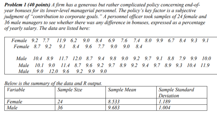
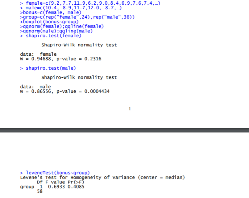
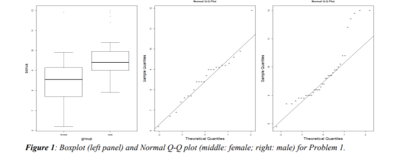
Problem 1 (40 points) A firm has a generous but rather complicated policy concerning end-of- year bonuses for its lower-level managerial personnel. The policy's key factor is a subjective judgment of contribution to corporate goals." A personnel officer took samples of 24 female and 36 male managers to see whether there was any difference in bonuses, expressed as a percentage of yearly salary. The data are listed here: Female 9.2 7.7 11.9 6.2 9.0 8.4 6.9 7.6 7.4 8.0 9.9 6.7 8.4 9.3 9.1 Female 8.7 9.2 9.1 8.4 9.6 7.7 9.0 9.0 8.4 Male 10.4 8.9 11.7 12.0 8.7 9.4 9.8 9.0 9.2 9.7 9.1 8.8 7.9 9.9 10.0 Male 10.1 9.0 11.4 8.7 9.6 9.2 9.7 8.9 9.2 9.4 9.7 8.9 9.3 10.4 11.9 Male 9.0 12.0 9.6 9.2 9.9 9.0 Below is the summary of the data and R output. Variable Sample Size Sample Mean Sample Standard Deviation 1.189 1.004 Female Male 24 36 8.533 9.683 > female=c(9.2,7.7,11.9,6.2,9.0,8.4,6.9,7.6.7.4, ...) > male=c(10.4, 8.9, 11.7,12.0, 8.7,-) >bonus=c(female, male) >group=C(rep ("female", 24), rep("male", 36)) >boxplot(bonus-group) >qqnorm(female); gline (female) >qqnorm (male);991ne (male) > Shapiro.test(female) Shapiro-wilk normality test data: female W = 0.94688, p-value = 0.2316 > shapiro.test(male) Shapiro-wilk normality test data: male W = 0.86556, p-value = 0.0004434 1 > leveneTest(bonus-group) Levene's Test for Homogeneity of variance (center = median) Df F value pr(>F) group 1 0.6933 0.4085 58 2 bonus Sampe Quanties Sample Quantes group Theoretical Quantiles Theoretical Quantiles Figure 1: Boxplot (left panel) and Normal Q-Q plot (middle: female; right: male) for Problem 1. Problem 1 (40 points) A firm has a generous but rather complicated policy concerning end-of- year bonuses for its lower-level managerial personnel. The policy's key factor is a subjective judgment of contribution to corporate goals." A personnel officer took samples of 24 female and 36 male managers to see whether there was any difference in bonuses, expressed as a percentage of yearly salary. The data are listed here: Female 9.2 7.7 11.9 6.2 9.0 8.4 6.9 7.6 7.4 8.0 9.9 6.7 8.4 9.3 9.1 Female 8.7 9.2 9.1 8.4 9.6 7.7 9.0 9.0 8.4 Male 10.4 8.9 11.7 12.0 8.7 9.4 9.8 9.0 9.2 9.7 9.1 8.8 7.9 9.9 10.0 Male 10.1 9.0 11.4 8.7 9.6 9.2 9.7 8.9 9.2 9.4 9.7 8.9 9.3 10.4 11.9 Male 9.0 12.0 9.6 9.2 9.9 9.0 Below is the summary of the data and R output. Variable Sample Size Sample Mean Sample Standard Deviation 1.189 1.004 Female Male 24 36 8.533 9.683 > female=c(9.2,7.7,11.9,6.2,9.0,8.4,6.9,7.6.7.4, ...) > male=c(10.4, 8.9, 11.7,12.0, 8.7,-) >bonus=c(female, male) >group=C(rep ("female", 24), rep("male", 36)) >boxplot(bonus-group) >qqnorm(female); gline (female) >qqnorm (male);991ne (male) > Shapiro.test(female) Shapiro-wilk normality test data: female W = 0.94688, p-value = 0.2316 > shapiro.test(male) Shapiro-wilk normality test data: male W = 0.86556, p-value = 0.0004434 1 > leveneTest(bonus-group) Levene's Test for Homogeneity of variance (center = median) Df F value pr(>F) group 1 0.6933 0.4085 58 2 bonus Sampe Quanties Sample Quantes group Theoretical Quantiles Theoretical Quantiles Figure 1: Boxplot (left panel) and Normal Q-Q plot (middle: female; right: male) for Problem 1