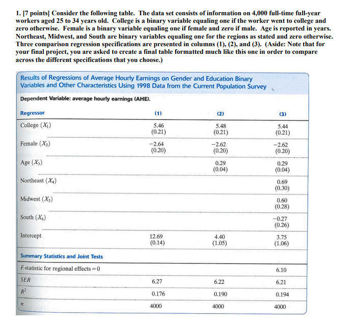
(a) Using the regression results in column (1), is the college-high school earnings difference estimated from this regression statistically significant at the 5% level? Use an appropriate statistical test to explain your answer. Show your work. (b) Using the regression results in column (1), is the male-female earnings difference estimated from this regression statistically significant at the 5% level? Use an appropriate statistical test to explain your answer. Show your work. (c) Using the regression results in column (2), is age an important determinant of earnings? Use an appropriate statistical test to explain your answer. Show your work. (d) Construct a 95% confidence interval for the expected difference between the earnings of a 29-year-old female college graduate and a 34-year old female college graduate. Show your work. (e) Using the regression results in column (3), do there appear to be important regional differences? Use an appropriate (joint) hypothesis test at the 1% level to explain your answer. Clearly explain what you are comparing in your test and the conclusions of your test. (f) What would happen if a regressor for the remaining region, West, was included? Explain why. (g) Compute R2 for each of the regression in columns (1)-(3). Show your work. (Hint: Think about how R- squared and adjusted R-squared are related. Specifically, think about how you can use the original R- squared given in the problem to calculate the adjusted R-squared.)1. [7 points] Consider the following table. The data set consists of information on 4,000 full-time full-year workers aged 25 to 34 years old. College is a binary variable equaling one if the worker went to college and zero otherwise. Female is a binary variable equaling one if female and zero if male. Age is reported in years. Northeast, Midwest, and South are binary variables equaling one for the regions as stated and zero otherwise. Three comparison regression specifications are presented in columns (1), (2), and (3). (Aside: Note that for your final project, you are asked to create a final table formatted much like this one in order to compare across the different specifications that you choose.) Results of Regressions of Average Hourly Earnings on Gender and Education Binary Variables and Other Characteristics Using 1998 Data from the Current Population Survey Dependent Variable: average hourly earnings (AHE). Regressor (1) (2) (3) College (X]) 5.46 5.48 (0.21) 5.44 (0.21) (0.21) Female (X2) -2.64 -2.62 -2.62 (0.20) (0.20) (0.20) Age (X,) 0.29 0.29 (0.04) (0.04) Northeast (X4) 0.69 (0.30) Midwest (Xs) 0.60 (0.28) South (X6) -0.27 (0.26) Intercept 12.69 4.40 3.75 (0.14) (1.05) (1.06) Summary Statistics and Joint Tests F-statistic for regional effects = 0 .10 SER 6.27 6.22 6.21 0.176 0.190 0.194 4000 4000 4000