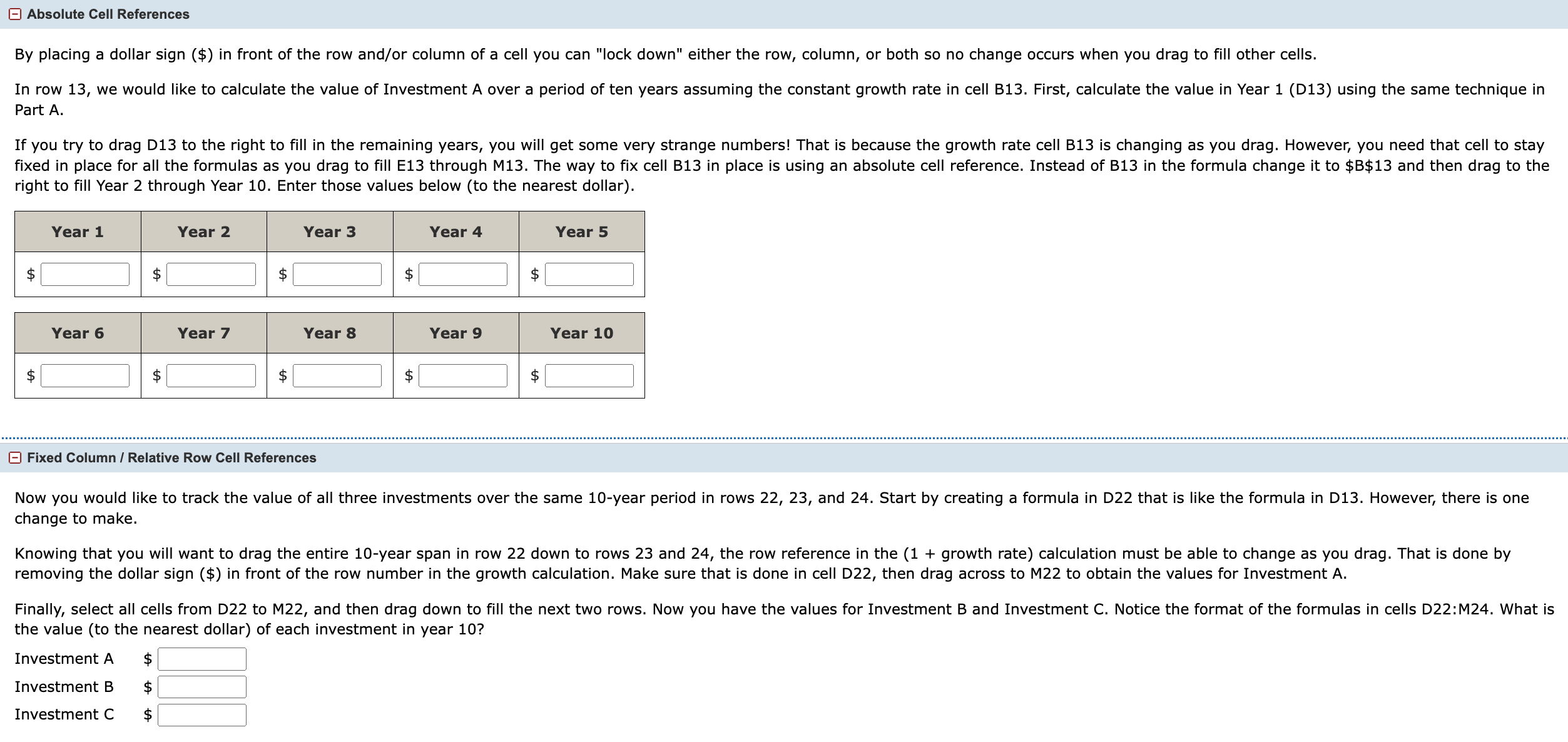
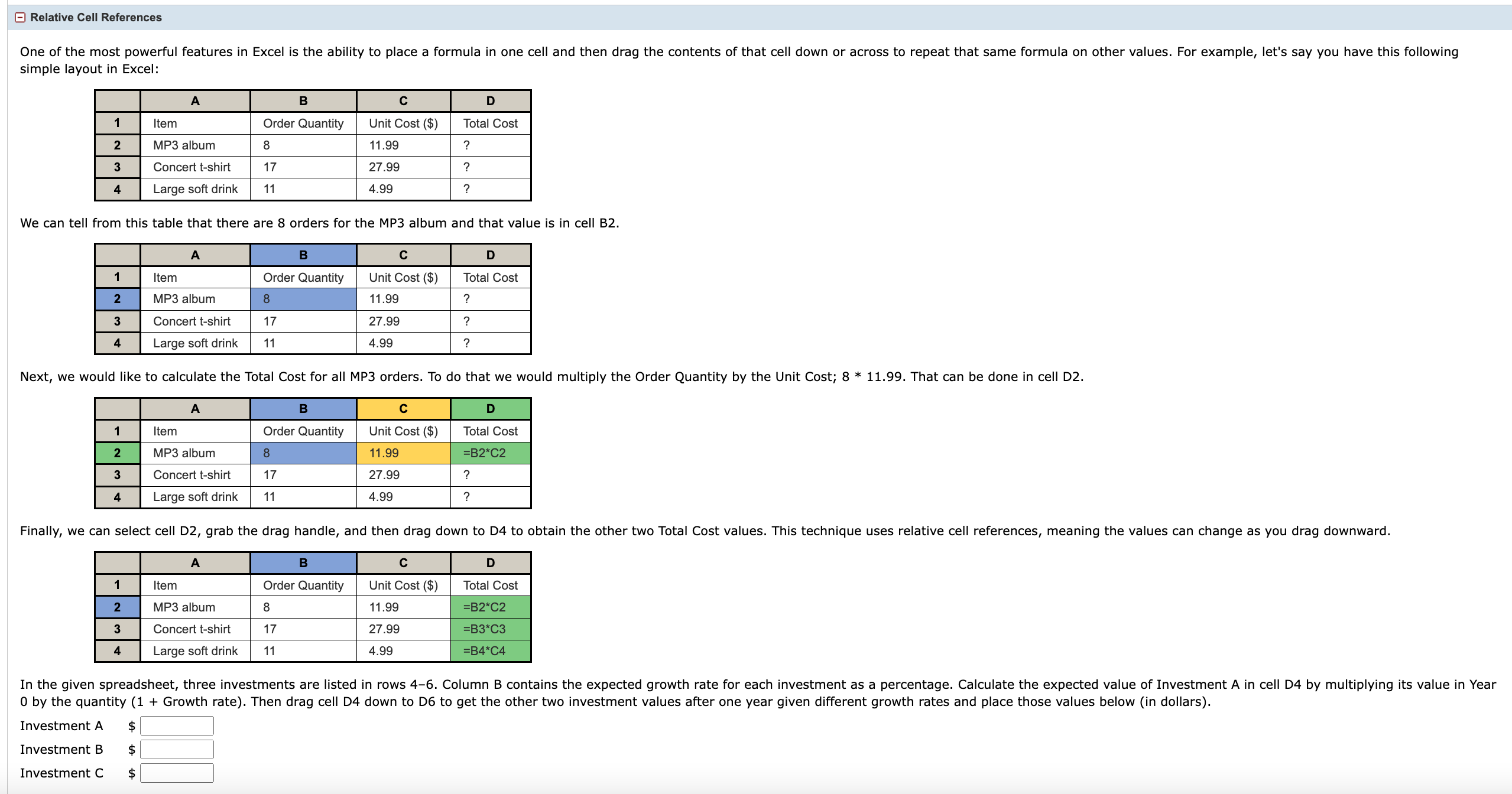
=) Absolute Cell References By placing a dollar sign ($) in front of the row and/or column of a cell you can "lock down" either the row, column, or both so no change occurs when you drag to fill other cells. In row 13, we would like to calculate the value of Investment A over a period of ten years assuming the constant growth rate in cell B13. First, calculate the value in Year 1 (D13) using the same technique in Part A. If you try to drag D13 to the right to fill in the remaining years, you will get some very strange numbers! That is because the growth rate cell B13 is changing as you drag. However, you need that cell to stay fixed in place for all the formulas as you drag to fill E13 through M13. The way to fix cell B13 in place is using an absolute cell reference. Instead of B13 in the formula change it to $B$13 and then drag to the right to fill Year 2 through Year 10. Enter those values below (to the nearest dollar). Year 1 Year 2 Year 3 Year 4 Year 5 $ I 8| Kl || [ J| s J Year 6 Year 7 Year 8 Year 9 Year 10 $ $| || s s $ (= Fixed Column / Relative Row Cell References Now you would like to track the value of all three investments over the same 10-year period in rows 22, 23, and 24. Start by creating a formula in D22 that is like the formula in D13. However, there is one change to make. Knowing that you will want to drag the entire 10-year span in row 22 down to rows 23 and 24, the row reference in the (1 + growth rate) calculation must be able to change as you drag. That is done by removing the dollar sign ($) in front of the row number in the growth calculation. Make sure that is done in cell D22, then drag across to M22 to obtain the values for Investment A. Finally, select all cells from D22 to M22, and then drag down to fill the next two rows. Now you have the values for Investment B and Investment C. Notice the format of the formulas in cells D22:M24. What is the value (to the nearest dollar) of each investment in year 10? Investment A | Investment B | Investment C $ = Relative Cell References One of the most powerful features in Excel is the ability to place a formula in one cell and then drag the contents of that cell down or across to repeat that same formula on other values. For example, let's say you have this following simple layout in Excel: Order Quantity | Unit Cost ($) MP3 album 8 11.99 Concert t-shirt 17 27.99 Large soft drink 1 4.99 We can tell from this table that there are 8 orders for the MP3 album and that value is in cell B2. Item Order Quantity Unit Cost ($) Total Cost MP3 album 11.99 ? Concert t-shirt 17 27.99 ? [ 4 | Largesoftarink [ 11 4.99 ? Item Order Quantity Unit Cost ($) Total Cost MP3 album 11.99 =B2*C2 Concert t-shirt 17 27.99 ? Large soft drink 1 4.99 2 Finally, we can select cell D2, grab the drag handle, and then drag down to D4 to obtain the other two Total Cost values. This technique uses relative cell references, meaning the values can change as you drag downward. Item Order Quantity Unit Cost ($) Total Cost MP3 album 8 11.99 =B2*C2 Concert t-shirt 17 27.99 =B3*C3 Large soft drink 11 4.99 =B4*C4 In the given spreadsheet, three investments are listed in rows 4-6. Column B contains the expected growth rate for each investment as a percentage. Calculate the expected value of Investment A in cell D4 by multiplying its value in Year 0 by the quantity (1 + Growth rate). Then drag cell D4 down to D6 to get the other two investment values after one year given different growth rates and place those values below (in dollars). Investment A $ Investment B $ Investment C $ \\ A B Ci D E E G H I J K L M N 1 2 Growth Rate | 3 (Expected) Year 0 Year 1 Formulas 4 |Investment A 1% $1,900 5 |Investment B 9% $1,900 6 |Investment C 1% $1,900 7/ 8 |"Take each value in column C and multiply it by its adjacent growth rate in column B (which is 1 plus the percentage expected growth)." 9 | = 10 | 11 _ Growth Rate I ) 12 (Expected) Year 0 Year 1 Year 2 Year 3 Year 4 Year 5 Year 6 Year 7 Year 8 Year 9 Year 10 | 13 Investment A 1% $1,900 | 14 15 |Formulas 16 17 "Startin column D, then move across allowing the column to change, and multiply the preceding value by its FIXED growth rate in cell $B$13 (which is 1 plus the percentage expected growth) to get the current value." 18 N 19! 20 Growth Rate L 21 (Expected) Year 0 Year 1 Year 2 Year 3 Year 4 Year 5 Year 6 Year7 Year 8 Year 9 Year 10 \\7 22 |Investment A 1% $1,900 . ; 23 Investment B 9% $1,900 [ 24 Investment C 1% $1,900 25 | 26 |Formulas 27 28 29 | 30 "Startin column D, then move across, and multiply the preceding value by its growth rate in cell $B22 (which is 1 plus the percentage expected growth) to get the cument value." B 31 "By changing the growth rate cell from $B$22, etc. to $B22, the row of the growth rate is allowed to change yet remain in column B while filing down to the other two Investments." 32 | L 33