1. Open PreBulkSales.xlsx. 2. Save the workbook using the name EL2-U1-A6-PreBulkSales. 3. Select A4:122 and create...

 

  

 

Transcribed Image Text:

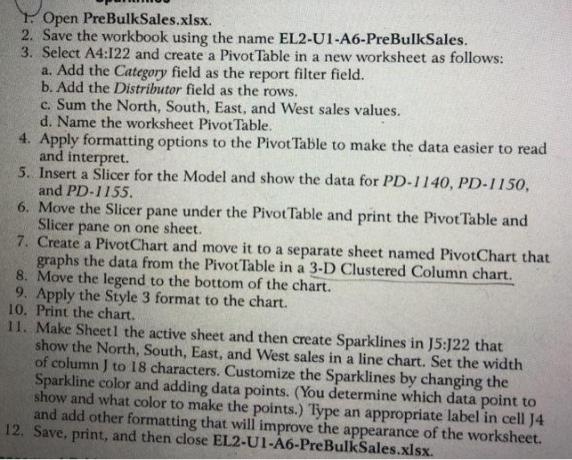
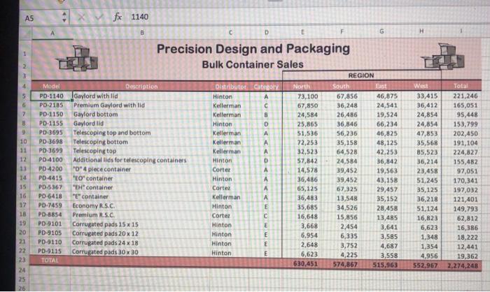
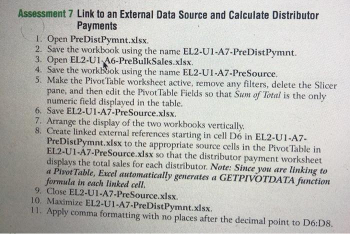
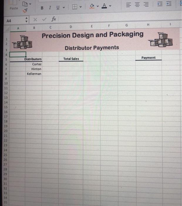
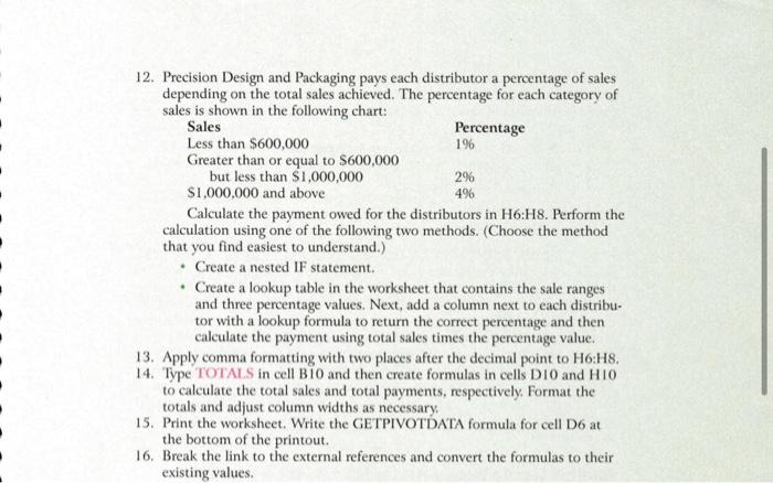
1. Open PreBulkSales.xlsx. 2. Save the workbook using the name EL2-U1-A6-PreBulkSales. 3. Select A4:122 and create a Pivot Table in a new worksheet as follows: a. Add the Category field as the report filter field. b. Add the Distributor field as the rows. c. Sum the North, South, East, and West sales values. d. Name the worksheet Pivot Table. 4. Apply formatting options to the Pivot Table to make the data easier to read and interpret. 5. Insert a Slicer for the Model and show the data for PD-1140, PD-1150, and PD-1155. 6. Move the Slicer pane under the Pivot Table and print the Pivot Table and Slicer pane on one sheet. 7. Create a PivotChart and move it to a separate sheet named PivotChart that graphs the data from the Pivot Table in a 3-D Clustered Column chart. 8. Move the legend to the bottom of the chart. 9. Apply the Style 3 format to the chart. 10. Print the chart. 11. Make Sheet1 the active sheet and then create Sparklines in J5:122 that show the North, South, East, and West sales in a line chart. Set the width of column J to 18 characters. Customize the Sparklines by changing the Sparkline color and adding data points. (You determine which data point to show and what color to make the points.) Type an appropriate label in cell J4 and add other formatting that will improve the appearance of the worksheet. 12. Save, print, and then close EL2-U1-A6-PreBulkSales.xlsx. A5 2 3 12 13 14 fx 1140 4 Model 5 PD-1140 Gaylord with lid 6 PD-2185 Premium Gaylord with lid 7 PD-1150 Gaylord bottom Gaylord lid 8 PD-1155 9 PD-3695 PD-3698 10 11 PD-3699 24 25 26 B Description Telescoping top and bottom Telescoping bottom PD-4100 PD-4200 "D" 4 piece container EO container PD-4415 15 PD-5367 16 PD-6418 18 19 17 PD-7459 Economy R.S.C. PD-8854 Premium R.S.C. PD-9101 Corrugated pads 15 x 15 20 PD-9105 Corrugated pads 20 x 12 21 PD-9110 Corrugated pads 24 x 18 22 PD-9115 Corrugated pads 30 x 30 23 TOTAL Telescoping top Additional lids for telescoping containers "EH"container "E"container C D Precision Design and Packaging Bulk Container Sales Distributor Category North Hinton A 73,100 C 67,850 8 24,584 Kellerman Kellerman Hinton Kellerman Kellerman 25,865 51,536 72,253 Kellerman 32,523 57,842 14,578 36,486 65,125 36,483 35,685 Hinton Cortez Hinton Cortez Kellerman Hinton Cortez Hinton Hinton Hinton Hinton D A A E A D A A A A E С E E E E F 16,648 3,668 6,954 2,648 6,623 630,451 REGION South 67,856 36,248 26,486 36,846 56,235 35,158 64,528 24,584 39,452 39,452 67,325 13,548 34,526 15,856 G East 46,875 24,541 19,524 66,234 46,825 48,125 42,253 36,842 19,563 43,158 29,457 35,152 28,458 13,485 2,454 3,641 6,335 3,585 3,752 4,687 4,225 3,558 574,867 515,963 H West 33,415 36,412 24,854 24,854 47,853 35,568 85,523 36,214 23,458 51,245 35,125 36,218 51,124 16,823 6,623 1,348 1,354 4,956 552,967 Total 221,246 165,051 95,448 153,799 202,450 191,104 224,827 155,482 97,051 170,341 197,032 121,401 149,793 62,812 16,386 18,222 12,441 19,362 2,274,248 Assessment 7 Link to an External Data Source and Calculate Distributor Payments 1. Open PreDistPymnt.xlsx. 2. Save the workbook using the name EL2-U1-A7-PreDistPymnt. 3. Open EL2-U1 A6-PreBulkSales.xlsx. 4. Save the workbook using the name EL2-U1-A7-PreSource. 5. Make the Pivot Table worksheet active, remove any filters, delete the Slicer pane, and then edit the Pivot Table Fields so that Sum of Total is the only numeric field displayed in the table. 6. Save EL2-U1-A7-PreSource.xlsx. 7. Arrange the display of the two workbooks vertically. 8. Create linked external references starting in cell D6 in EL2-U1-A7- PreDistPymnt.xlsx to the appropriate source cells in the Pivot Table in EL2-U1-A7-PreSource.xlsx so that the distributor payment worksheet displays the total sales for each distributor. Note: Since you are linking to a Pivot Table, Excel automatically generates a GETPIVOTDATA function formula in each linked cell. 9. Close EL2-U1-A7-PreSource.xlsx. 10. Maximize EL2-U1-A7-PreDistPymnt.xlsx. 11. Apply comma formatting with no places after the decimal point to D6:D8. A4 1234567 H 8 9 10 11 12 13 15 16 17 18 19 20 21 22 23 24 25 26 27 28 29 30 31 LAWN5 Paste 32 33 34 35 A AY 16 V BIU. x ✓ fx B Distributors Cortez Hinton Kellerman C V D Total Sales G Precision Design and Packaging Distributor Payments E A F 三三三三 E H Payment TEST 12. Precision Design and Packaging pays each distributor a percentage of sales depending on the total sales achieved. The percentage for each category of sales is shown in the following chart: Sales Less than $600,000 Greater than or equal to $600,000 but less than $1,000,000 $1,000,000 and above Percentage 196 2% 4% Calculate the payment owed for the distributors in H6:H8. Perform the calculation using one of the following two methods. (Choose the method that you find easiest to understand.) • Create a nested IF statement. • Create a lookup table in the worksheet that contains the sale ranges and three percentage values. Next, add a column next to each distribu- tor with a lookup formula to return the correct percentage and then calculate the payment using total sales times the percentage value. 13. Apply comma formatting with two places after the decimal point to H6:H8. 14. Type TOTALS in cell B10 and then create formulas in cells D10 and H10 to calculate the total sales and total payments, respectively. Format the totals and adjust column widths as necessary. 15. Print the worksheet. Write the GETPIVOTDATA formula for cell D6 at the bottom of the printout. 16. Break the link to the external references and convert the formulas to their existing values. 1. Open PreBulkSales.xlsx. 2. Save the workbook using the name EL2-U1-A6-PreBulkSales. 3. Select A4:122 and create a Pivot Table in a new worksheet as follows: a. Add the Category field as the report filter field. b. Add the Distributor field as the rows. c. Sum the North, South, East, and West sales values. d. Name the worksheet Pivot Table. 4. Apply formatting options to the Pivot Table to make the data easier to read and interpret. 5. Insert a Slicer for the Model and show the data for PD-1140, PD-1150, and PD-1155. 6. Move the Slicer pane under the Pivot Table and print the Pivot Table and Slicer pane on one sheet. 7. Create a PivotChart and move it to a separate sheet named PivotChart that graphs the data from the Pivot Table in a 3-D Clustered Column chart. 8. Move the legend to the bottom of the chart. 9. Apply the Style 3 format to the chart. 10. Print the chart. 11. Make Sheet1 the active sheet and then create Sparklines in J5:122 that show the North, South, East, and West sales in a line chart. Set the width of column J to 18 characters. Customize the Sparklines by changing the Sparkline color and adding data points. (You determine which data point to show and what color to make the points.) Type an appropriate label in cell J4 and add other formatting that will improve the appearance of the worksheet. 12. Save, print, and then close EL2-U1-A6-PreBulkSales.xlsx. A5 2 3 12 13 14 fx 1140 4 Model 5 PD-1140 Gaylord with lid 6 PD-2185 Premium Gaylord with lid 7 PD-1150 Gaylord bottom Gaylord lid 8 PD-1155 9 PD-3695 PD-3698 10 11 PD-3699 24 25 26 B Description Telescoping top and bottom Telescoping bottom PD-4100 PD-4200 "D" 4 piece container EO container PD-4415 15 PD-5367 16 PD-6418 18 19 17 PD-7459 Economy R.S.C. PD-8854 Premium R.S.C. PD-9101 Corrugated pads 15 x 15 20 PD-9105 Corrugated pads 20 x 12 21 PD-9110 Corrugated pads 24 x 18 22 PD-9115 Corrugated pads 30 x 30 23 TOTAL Telescoping top Additional lids for telescoping containers "EH"container "E"container C D Precision Design and Packaging Bulk Container Sales Distributor Category North Hinton A 73,100 C 67,850 8 24,584 Kellerman Kellerman Hinton Kellerman Kellerman 25,865 51,536 72,253 Kellerman 32,523 57,842 14,578 36,486 65,125 36,483 35,685 Hinton Cortez Hinton Cortez Kellerman Hinton Cortez Hinton Hinton Hinton Hinton D A A E A D A A A A E С E E E E F 16,648 3,668 6,954 2,648 6,623 630,451 REGION South 67,856 36,248 26,486 36,846 56,235 35,158 64,528 24,584 39,452 39,452 67,325 13,548 34,526 15,856 G East 46,875 24,541 19,524 66,234 46,825 48,125 42,253 36,842 19,563 43,158 29,457 35,152 28,458 13,485 2,454 3,641 6,335 3,585 3,752 4,687 4,225 3,558 574,867 515,963 H West 33,415 36,412 24,854 24,854 47,853 35,568 85,523 36,214 23,458 51,245 35,125 36,218 51,124 16,823 6,623 1,348 1,354 4,956 552,967 Total 221,246 165,051 95,448 153,799 202,450 191,104 224,827 155,482 97,051 170,341 197,032 121,401 149,793 62,812 16,386 18,222 12,441 19,362 2,274,248 Assessment 7 Link to an External Data Source and Calculate Distributor Payments 1. Open PreDistPymnt.xlsx. 2. Save the workbook using the name EL2-U1-A7-PreDistPymnt. 3. Open EL2-U1 A6-PreBulkSales.xlsx. 4. Save the workbook using the name EL2-U1-A7-PreSource. 5. Make the Pivot Table worksheet active, remove any filters, delete the Slicer pane, and then edit the Pivot Table Fields so that Sum of Total is the only numeric field displayed in the table. 6. Save EL2-U1-A7-PreSource.xlsx. 7. Arrange the display of the two workbooks vertically. 8. Create linked external references starting in cell D6 in EL2-U1-A7- PreDistPymnt.xlsx to the appropriate source cells in the Pivot Table in EL2-U1-A7-PreSource.xlsx so that the distributor payment worksheet displays the total sales for each distributor. Note: Since you are linking to a Pivot Table, Excel automatically generates a GETPIVOTDATA function formula in each linked cell. 9. Close EL2-U1-A7-PreSource.xlsx. 10. Maximize EL2-U1-A7-PreDistPymnt.xlsx. 11. Apply comma formatting with no places after the decimal point to D6:D8. A4 1234567 H 8 9 10 11 12 13 15 16 17 18 19 20 21 22 23 24 25 26 27 28 29 30 31 LAWN5 Paste 32 33 34 35 A AY 16 V BIU. x ✓ fx B Distributors Cortez Hinton Kellerman C V D Total Sales G Precision Design and Packaging Distributor Payments E A F 三三三三 E H Payment TEST 12. Precision Design and Packaging pays each distributor a percentage of sales depending on the total sales achieved. The percentage for each category of sales is shown in the following chart: Sales Less than $600,000 Greater than or equal to $600,000 but less than $1,000,000 $1,000,000 and above Percentage 196 2% 4% Calculate the payment owed for the distributors in H6:H8. Perform the calculation using one of the following two methods. (Choose the method that you find easiest to understand.) • Create a nested IF statement. • Create a lookup table in the worksheet that contains the sale ranges and three percentage values. Next, add a column next to each distribu- tor with a lookup formula to return the correct percentage and then calculate the payment using total sales times the percentage value. 13. Apply comma formatting with two places after the decimal point to H6:H8. 14. Type TOTALS in cell B10 and then create formulas in cells D10 and H10 to calculate the total sales and total payments, respectively. Format the totals and adjust column widths as necessary. 15. Print the worksheet. Write the GETPIVOTDATA formula for cell D6 at the bottom of the printout. 16. Break the link to the external references and convert the formulas to their existing values.