Activity 4 Full Assignment

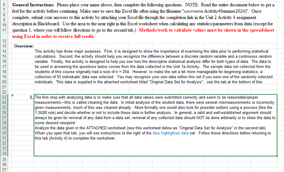
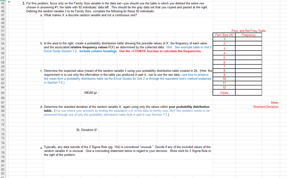
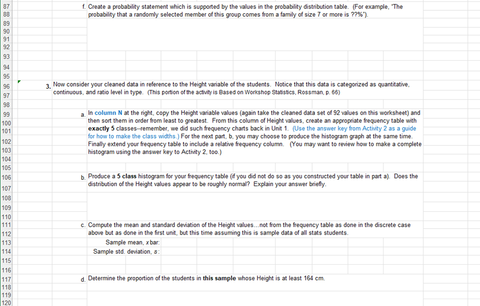
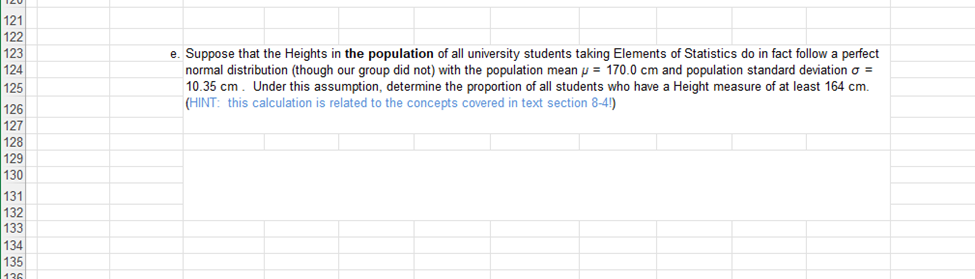
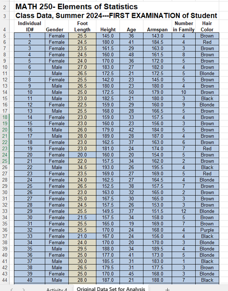
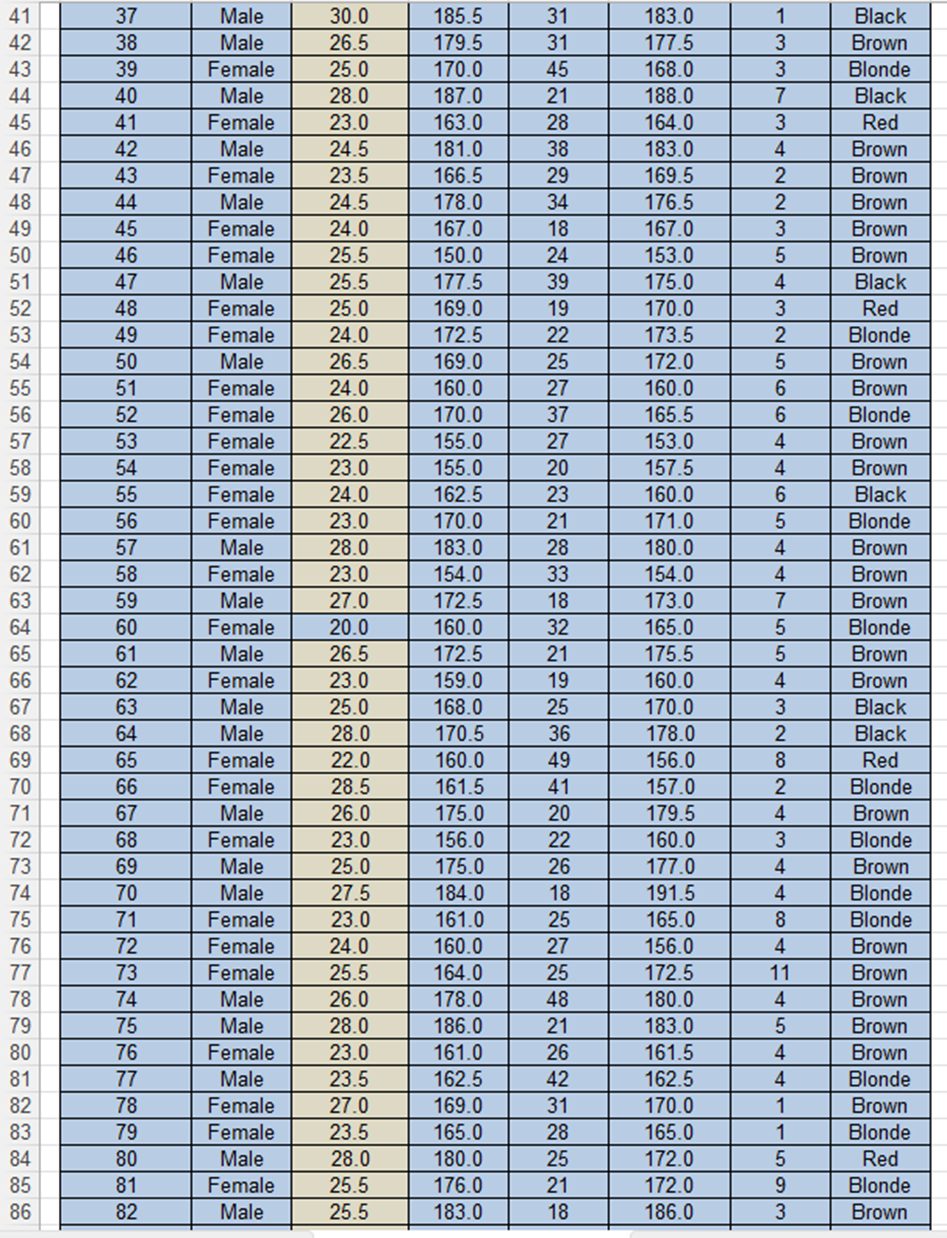
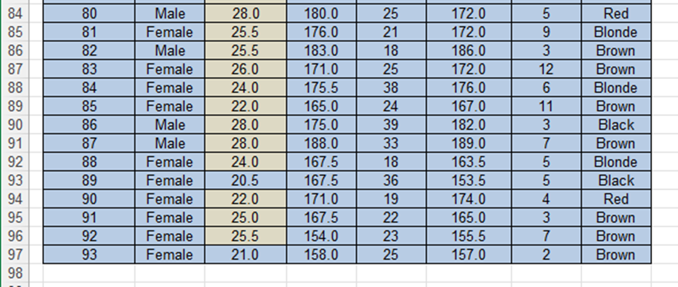
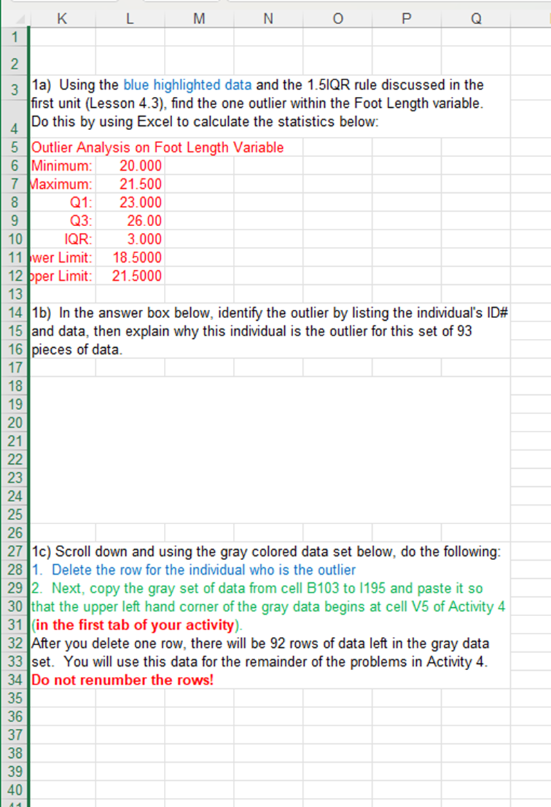
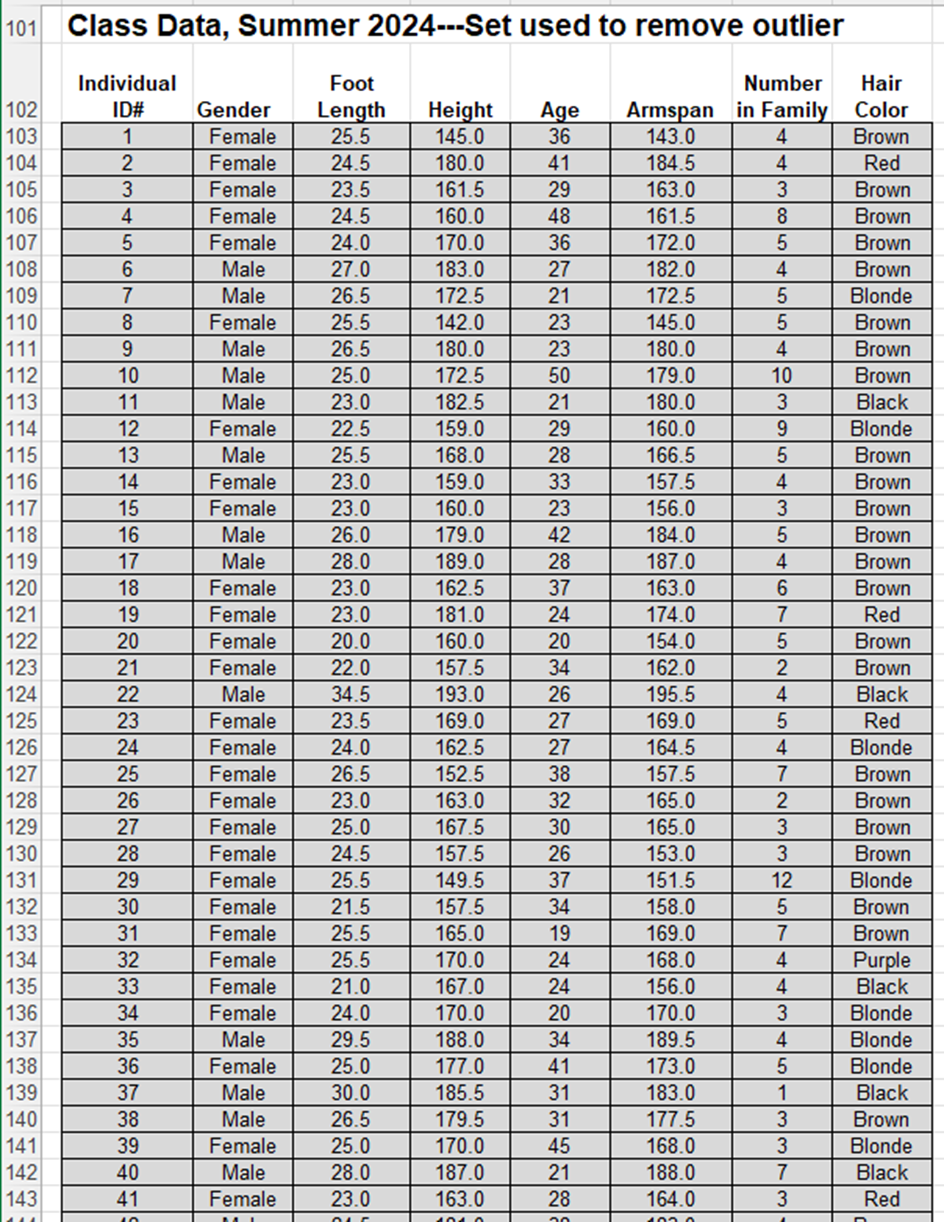
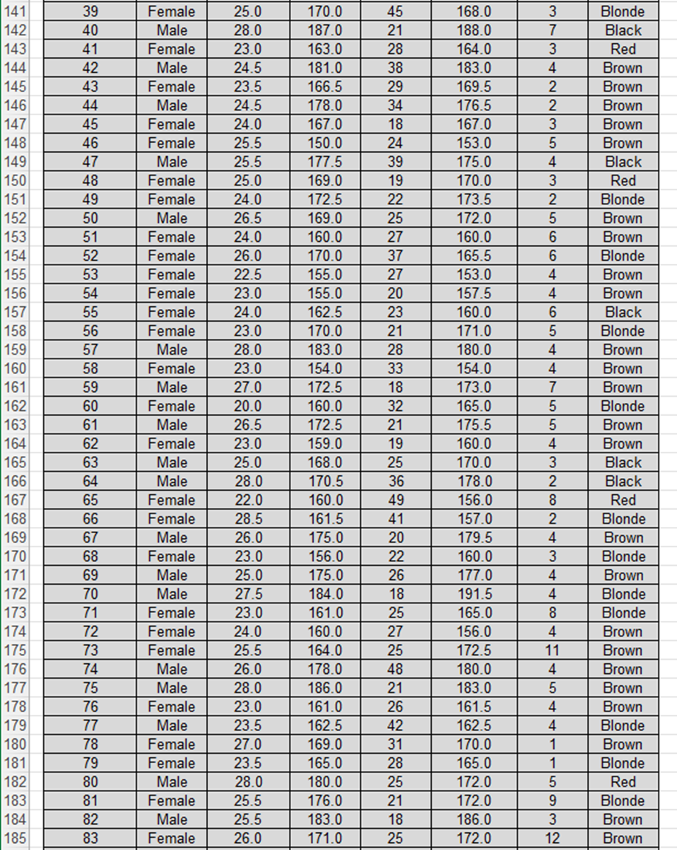
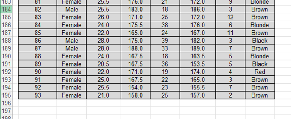
General Instructions: Please place your name above, then complete the following questions. NOTE: Read the entire document below to geta feel for the activity before continning. Make sure to save this Excel file often using the filename "voirname Activity4Summer2024)". Once complete, submit your answers to this activity by attaching your Excel file through the completion link in the Unit 2 Activity 4 assignment description in Blackboard. Use the area to the near right in this Excel worksheet when calculating any statistics/parameters from data (except for question 1, where you will follow directions to go to the second tab.) Methods/work to calculate values must be shown in the spreadsheet using Excel in order to receive full credit. Overview: This actiity has three major purposes. First, it is designed to show the importance of examining the data prior to performing statistical calculations. Second, the actiity should help you recognize the difference between a discrete random variable and a continuous random variable. Finally, the activity is designed to help you see how the descriptive statistical analysis differ for both types of data. The data to be used in answering the questions below comes from the data collected in the Unit 1a Actiity. The sample data set collected from the students of this course originally had a size of n = 254. However, to make the set a bit more manageable for beginning statistics, a collection of 93 individuals' data was selected. You may recognize your own data within this set if you were one of the randomly selected individuals. This data is supplied in the attached worksheet titled "Original Data Set for Analysis\"...see the tab at the bottom of this .| The first step with analyzing data is to make sure that all data values were submitted cormrectly and seem to be reasonable/proper measurementsthis is called cleaning the data. In initial analysis of the student data, there were several mismeasurements or incorrectly given measurements; much of this was cleaned already. More formally one would also look for possible outliers using a process (like the 1.51QR rule) and decide whether or not to include these data in further analysis. In general, a valid and well-established argument should always be given for removal of any data from a data set; removal of any collected data should NOT be done arbitranily or to skew the data to some desired viewpoint. Analyze the data given in the ATTACHED worksheet (see this worksheet below as "Original Data Set for Analysis\" in the second tab) When you open that tab, you will see instructions to the right of the blue highlighted data set. Follow those directions before returning to this tab (Activity 4) to complete the worksheet. 45 46 a7 48 49 50 51 52 53 55 56 57 58 59 60 61 62 63 65 66 67 68 69 70 4| 72 73 74 75 76 T 78 79 80 8 82 83 oa 2. For this problem, focus only on the Family Size variable in the data setyou should use the table in which you deleted the entire row chosen in answering #1; the table with 92 indmduals' data left. This should be the gray data set that you copied and pasted at the night Defining the random variable X to be Family Size. complete the following for these 92 indmduals: a What makes X a discrete random variable and not a continuous one? Freq. and Rel.Freq. Table | Fam Size (%) | Frequency | .+ 1 b. In the area to the right, create a probability distribution table showing the possible values of X, the frequency of eachvalue, [ 2 [ ] and the associated relative frequency values P(X) as determined by the collected data. Hint: See example table in Unit 2 _ Excel Guide Section 7.2. Include column headings. Use the =COUNTIF function to calculate the frequencies. 7 1 ] . Determine the expected value (mean) of the random variable X using your probability distribution table createdin2b. (Hint:the] 8 [ ] requirement is to use only the information in the table you produced in part b., not to use the raw datasee howtoproduce | 9 | | the mean from a probability distribution table via the Excel Guides for Unit 2 or through the equivalent text's method explained [ 10 | | in Section 7-2.) [ | % MEAN [ tows | | d. Determine the standard desiation of the random variable X, again using only the values within your probability distribution Standard Deviation: naeds to be table. (You can check your answers by the population 5.d. of the data on fz s BUT this prc answered through use of only th I St. Deviation 0 o Typically, any data outside of the 2 Sigma Rule (pg. 154) is considered \"unusual.\" Decide if any of the included values of the random variable X is unusual. Give a concluding statement below in regard to your decision. Show work for 2 Sigma Rule to the nght of the problem. 87 f. Create a probability statement which is supported by the values in the probability distribution table. {For example, \"The 88 | probability that a randomly selected member of this group comes from a family of size 7 or more is 77%"). 89 90| 91 | 92 93| 94 95 | 9% 3. Mow consider your cleaned data in reference to the Height vanable of the students. Motice that this data is categorized as quantitative, 97 continuous, and ratio level in type. (This portion of the activity is Based on Workshop Statistics, Rossman, p. 66) 98 99 | 3. In column N at the right, copy the Height variable values (again take the cleaned data set of 92 values on this worksheet) and 100/ then sort them in order from least to greatest. From this column of Height values, create an appropriate frequency table with 101/ exactly 5 classesremember, we did such frequency charts back in Unit 1. (Use the answer key from Actiity 2 as a guide | for how to make the class widths.) For the next part, b, you may choose to produce the histogram graph at the same time. 102 Finally extend your frequency table to include a relative frequency column. (You may want to review how to make a complete 103 histogram using the answer key to Activity 2, too.) 104 105 106 p. Produce a 5 class histogram for your frequency table (if you did not do so as you constructed your table in part a). Does the 10?' distribution of the Height values appear to be roughly normal? Explain your answer briefly. 108| 109| 110 111] c. Compute the mean and standard deviation of the Height values...not from the frequency table as done in the discrete case 112 above but as done in the first unit, but this time assuming this is sample data of all stats students. 113 Sample mean, xbar: 114 Sample std. deviation, s: 115 116 117 d. Determine the proportion of the students in this sample whose Height is at least 164 cm. 118| 119| 120 121 122 123 124 125| 126| 127 128| 129 130| 131| 132 133| 134| 135| 128 e. Suppose that the Heights in the population of all university students taking Elements of Statistics do in fact follow a perfect normal distribution (though our group did not) with the population mean g = 170.0 cm and population standard deviation o = 10.35 cm . Under this assumption, determine the proportion of all students who have a Height measure of at least 164 cm. (HINT: this calculation is related to the concepts covered in text section 8-41) R S T U V W X Y Z AA AB AC AD MATH 250- Elements of Statistics W N Class Data, Summer 2024---CLEANED Student Data Individual Number in Hair ID# Gender Foot Length Height Age Armspan Family ColorN MATH 250- Elements of Statistics W Class Data, Summer 2024---FIRST EXAMINATION of Student Individual Foot Number Hair ID# Gender Length Height Age Armspan in Family Color 1 Female 25.5 145.0 36 143.0 4 Brown Female 24.5 180.0 41 184.5 Red Female 23.5 161.5 29 163.0 Brown OM AWN Female 24.5 160.0 48 161.5 Brown Female 24.0 170.0 36 172.0 Brown A CI CI A CI OO W A Male 27.0 183.0 27 182.0 Brown Male 26.5 172.5 21 172.5 Blonde Female 25.5 142.0 23 145.0 Brown Male 26.5 180.0 23 180.0 Brown 10 Male 25.0 172.5 50 179.0 10 Brown 11 Male 23.0 182.5 21 180.0 3 Black 12 Female 22.5 159.0 29 160.0 Blonde 13 Male 25.5 168.0 28 166.5 Brown 14 Female 23.0 159.0 33 157.5 Brown 19 15 Female 23.0 160.0 23 156.0 Brown 20 16 Male 26.0 179.0 42 184.0 Brown 21 17 Male 28.0 189.0 28 187.0 Brown 22 18 Female 23.0 162.5 37 163.0 6 Brown 23 19 Female 23.0 181.0 24 174.0 Red 24 20 Female 20.0 160.0 20 154.0 Brown 25 21 Female 22.0 157.5 34 162.0 Brown 26 22 Male 34.5 193.0 26 195.5 Black 27 23 Female 23.5 169.0 27 169.0 Red 28 24 Female 24.0 162.5 27 164.5 Blonde 29 25 Female 26.5 152.5 38 157.5 Brown 30 26 Female 23.0 163.0 32 165.0 Brown 31 27 Female 25.0 167.5 30 165.0 Brown 32 28 Female 24.5 157.5 26 153.0 3 Brown 33 29 Female 25.5 149.5 37 151.5 12 Blonde 34 30 Female 21.5 157.5 34 158.0 Brown 35 31 Female 25.5 165.0 19 169.0 Brown 36 32 Female 25.5 170.0 24 168.0 Purple 37 33 Female 21.0 167.0 24 156.0 Black 38 34 Female 24.0 170.0 20 170.0 3 Blonde 39 35 Male 29.5 188.0 34 189.5 4 Blonde 40 36 Female 25.0 177.0 41 173.0 5 Blonde 41 37 Male 30.0 185.5 31 183.0 Black 42 38 Male 26.5 179.5 31 177.5 w w - Brown 43 39 Female 25.0 170.0 45 168.0 Blonde 44 40 Male 28.0 187.0 21 188.0 Black Original Data Set for Analysis41 37 Male 30.0 185.5 31 183.0 Black 42 38 Male 26.5 179.5 31 177.5 Brown - w w - 43 39 Female 25.0 170.0 45 168.0 Blonde 44 40 Male 28.0 187.0 21 188.0 Black 45 41 Female 23.0 163.0 28 164.0 3 Red 46 42 Male 24.5 181.0 38 183.0 Brown 47 43 Female 23.5 166.5 29 169.5 NN A Brown 48 44 Male 24.5 178.0 34 176.5 Brown 49 45 Female 24.0 167.0 18 167.0 3 Brown 50 46 Female 25.5 150.0 24 153.0 5 Brown 51 47 Male 25.5 177.5 39 175.0 Black W A 52 48 Female 25.0 169.0 19 170.0 Red 53 49 Female 24.0 172.5 22 173.5 2 Blonde 54 50 Male 26.5 169.0 25 172.0 5 Brown 55 51 Female 24.0 160.0 27 160.0 Brown 56 52 Female 26.0 170.0 37 165.5 6 Blonde 57 53 Female 22.5 155.0 27 153.0 Brown 58 54 Female 23.0 155.0 20 157.5 Brown 59 55 Female 24.0 162.5 23 160.0 6 Black 60 56 Female 23.0 170.0 21 171.0 5 Blonde 61 57 Male 28.0 183.0 28 180.0 Brown 62 58 Female 23.0 154.0 33 154.0 Brown 63 59 Male 27.0 172.5 18 173.0 Brown 64 60 Female 20.0 160.0 32 165.0 Blonde 65 61 Male 26.5 172.5 21 175.5 Brown 66 62 Female 23.0 159.0 19 160.0 Brown 67 63 Male 25.0 168.0 25 170.0 Black 68 64 Male 28.0 170.5 36 178.0 Black 69 65 Female 22.0 160.0 49 156.0 Red 70 66 Female 28.5 161.5 41 157.0 WANOON Blonde 71 67 Male 26.0 175.0 20 179.5 Brown 72 68 Female 23.0 156.0 22 160.0 Blonde 73 69 Male 25.0 175.0 26 177.0 Brown 74 70 Male 27.5 184.0 18 191.5 Blonde 75 71 Female 23.0 161.0 25 165.0 8 Blonde 76 72 Female 24.0 160.0 27 156.0 4 Brown 77 73 Female 25.5 164.0 25 172.5 11 Brown 78 74 Male 26.0 178.0 48 180.0 4 Brown 79 75 Male 28.0 186.0 21 183.0 5 Brown 80 76 Female 23.0 161.0 26 161.5 Brown 81 77 Male 23.5 162.5 42 162.5 Blonde 82 78 Female 27.0 169.0 31 170.0 Brown 83 79 Female 23.5 165.0 28 165.0 1 Blonde 84 80 Male 28.0 180.0 25 172.0 5 Red 85 81 Female 25.5 176.0 21 172.0 9 Blonde 86 82 Male 25.5 183.0 18 186.0 3 Brown\"mm 1800 | 25 | 1720 | 6 | Red | | 81 [ Female | 256 | 1760 [ 21 | 1720 [ 9 [ Blonde | | 82 [ 255 | : | Brown | 88 [ Female | 240 | 1675 | 18 | 1635 | 89 | Female | 205 | 1675 | 3 | 1535 [ 5 | Black | | 90 | Female | 220 [ 1710 [ 19 | 1740 [ 4 | Red | | 91 | Female | 250 | 1675 | 22 | 1650 [ 3 | Brown | | 92 [Female | 265 | 1540 | 23 | 1565 | 7 | Brown | | 93 [ Female | 210 [ 1580 | 25 | 1570 [ 2 | Brown | |1a) Using the blue highlighted data and the 1.51QR rule discussed in the |first unit (Lesson 4.3), find the one outlier within the Foot Length variable. Do this by using Excel to calculate the statistics below: |Outlier Analysis on Foot Length Variable {Minimum: ~ 20.000 aximum: 21.500 Q1: 23.000 Q3: 26.00 IQR: 3.000 Bwer Limit: 18.5000 Ppper Limit: 21.5000 : 1b) In the answer box below, identify the outlier by listing the individual's ID# |and data, then explain why this individual is the outlier for this set of 93 pieces of data. 1c) Scroll down and using the gray colored data set below, do the following: |1. Delete the row for the individual who is the outlier J2. Next, copy the gray set of data from cell B103 to 1195 and paste it so | Jthat the upper left hand corner of the gray data begins at cell V5 of Activity 4 |(in the first tab of your activity) After you delete one row, there will be 92 rows of data left in the gray data |set. You will use this data for the remainder of the problems in Activity 4. Do not renumber the rows! 101 102 103 104 105 106 107 108 109 110 111 112 113 114 115 116 117 118 119 120 121 122 123 124 125 126 127 128 129 130 131 132 133 134 135 136 137 138 139 140 141 142 143 Class Data, Summer 2024---Set used to remove outlier Individual Foot Number Hair ID# Gender Length Height Age Armspan in Family Color _-lm | 2 [Female | 245 | 1800 | 41 | 1845 | 4 | Red | | 3 | Female | 235 | 1615 | 29 | 1630 | 3 | Brown | | 4 | Female | 245 | 1600 | 48 | 1615 | 8 | Brown | | 5 | Female [ 240 | 1700 | 36 | 1720 | 5 | Brown | | 6 | Male | 270 | 1830 | 27 | 1820 | 4 | Brown | | 7 | Male | 265 | 1725 | 21 | 1725 | 5 | Blonde | | 8 | Female | 255 | 1420 | 23 | 1450 | 5 | Brown | | 9 | Male | 265 | 1800 | 23 | 1800 | 4 | Brown | | 10 | Male | 250 | 1725 | 50 | 1790 | 10 | Brown | | 11 | Male | 230 | 1825 | 21 | 1800 | 3 | Black | | 12 [Female | 225 | 1590 | 29 | 1600 | 9 | Blonde | | 13 | Male | 255 | 1680 | 28 | 1665 | 5 | Brown | | 14 [Female [ 230 | 1590 | 33 | 1575 | 4 | Brown | | 15 [ Female | 230 | 1600 | 23 | 1560 | 3 | Brown | | 16 | Male | 260 | 1790 | 42 | 1840 | 5 | Brown | | 17 | Male | 280 | 1890 | 28 | 1870 | 4 | Brown | | 18 [Female | 230 | 1625 | 37 | 1630 | 6 | Brown | | 19 [Female | 230 | 1810 | 24 | 1740 | 7 | Red | | 20 [ Female | 200 | 1600 | 20 | 1540 | 5 | Brown | | 21 [Female [ 220 | 1575 | 34 | 1620 | 2 | Brown | | 22 | Male | 345 | 1930 | 26 | 1955 | 4 | Black | | 23 | Female | 235 | 1690 | 27 | 1690 | 5 | Red | | 24 [ Female | 240 | 1625 | 27 | 1645 | 4 | Blonde | | 25 [Female | 265 | 1525 | 38 | 15756 | 7 | Brown | | 26 [ Female | 230 | 1630 | 32 | 1650 | 2 | Brown | | 27 | Female | 250 | 1675 | 30 | 1650 | 3 | Brown | | 28 [ Female | 245 | 1575 | 26 | 1530 | 3 | Brown | | 30 [Female [ 215 | 1575 | 34 | 1580 | 5 | Brown | | 31 [Female | 255 | 1650 | 19 | 1690 | 7 | Brown | | 32 [Female | 265 | 1700 | 24 | 1680 | 4 | Purple | | 33 |[Female | 210 | 1670 | 24 | 1560 | 4 | Black | | 34 | Female | 240 | 1700 | 20 | 1700 | 3 | Blonde | | 35 | Male | 295 | 1880 | 34 | 1895 | 4 | Blonde | | 36 | Female | 250 | 1770 | 41 | 1730 | 5 | Blonde | | 37 | Male | 300 | 1855 | 31 | 1830 | 1 | Black | | 38 | Male | 265 | 1795 | 31 | 1775 | 3 | Brown | | 39 |Female | 250 | 1700 | 45 | 1680 | 3 | Blonde | | 40 | Male | 280 | 1870 | 21 | 180 | 7 | Black | | 41 [Female [ 230 [ 1630 [ 28 [ 1640 | 3 | Red | | 39 | Female | 250 | 1700 | 45 | 1680 | 3 | Blonde | | 40 | Male | 280 | 1870 | 21 | 1880 [ 7 | Black | | 41 [ Female | 230 | 1630 | 28 | 1640 | 3 | Red | [ 42 | Male | 245 | 1810 | 38 | 1830 | 4 | Brown | | 43 | Female | 235 | 1665 | 29 | 1695 | 2 | Brown | 44 | Male | 245 | 1780 | 34 | 1765 | 2 | Brown | | 45 | Female | 240 | 1670 | 18 | 1670 | 3 | Brown | | 46 | Female | 255 | 1500 | 24 | 1530 | 5 | Brown | 47 | Male | 265 | 1775 | 39 | 1750 | 4 | Black | | 48 | Female | 250 | 1690 | 19 | 1700 | 3 | Red | | 49 | Female | 240 | 1725 | 22 | 1735 | 2 | Blonde | | 50 | Male | 265 | 1690 | 256 | 1720 | 5 | Brown | | 51 | Female | 240 | 1600 | 27 | 1600 | 6 | Brown | | 52 | Female | 260 | 1700 | 37 | 1655 | 6 | Blonde | | 53 | Female | 225 | 1550 | 27 | 1530 | 4 | Brown | | 54 | Female | 230 | 1550 | 20 | 1575 | 4 | Brown | | 55 | Female | 240 | 1625 | 23 | 1600 | 6 | Black | | 56 | Female | 230 | 1700 | 21 | 1710 [ 5 | Blonde | | 57 | Male | 280 | 1830 | 28 | 1800 | 4 | Brown | | 58 | Female | 230 | 1540 | 33 | 1540 | 4 | | 59 | Male | 270 | 1725 | 18 | 1730 | 7 | Brown | | 60 |Female | 200 | 1600 | 32 | 1650 | 5 | Blonde | | 61 | Male | 265 | 1725 | 21 | 1755 | 5 | Brown | | 62 | Female | 230 | 1590 | 19 | 1600 | 4 | Brown | 63 | Male | 250 | 1680 [ 25 | 1700 [ 3 | Black | | 64 | Male | 280 | 1705 | 36 | 1780 | 2 | Black | | 65 | Female | 220 | 1600 | 49 | 1560 | 8 | Red | | 66 | Female | 285 | 1615 | 41 | 1570 | 2 | Blonde | | 67 | Male | 260 | 1750 | 20 | 1795 | 4 | Brown | 68 | Female | 230 | 1560 | 22 | 1600 [ 3 | Blonde | | 69 | Male | 250 | 1750 | 26 | 1770 | 4 | Brown | 70 | Male | 275 | 1840 [ 18 | 1915 [ 4 | Blonde | m\" | 72 | Female | 240 | 1600 | 27 | 1560 | 4 | Brown | [ 73 [Female | 255 | 1640 | 26 | 1725 [ 11 | Brown | 74 | Male | 260 | 1780 | 48 | 1800 | 4 | Brown | | 75 | Male | 280 | 1860 | 21 | 1830 | 5 | Brown | | 76 [ Female | 230 | 1610 | 26 | 1615 | 4 | Brown -mmm-m-- | 78 | Female | 27.0 | 1690 | 31 | 1700 | 1 | Brown | | 79 | Female | 235 | 1650 | 28 | 1650 | 1 | Blonde | | 80 | Male | 280 | 1800 | 25 | 1720 | 5 | Red | | 81 [Female | 255 | 1760 | 21 | 1720 | 9 | Blonde | 82 | Male | 265 | 1830 [ 18 | 1860 [ 3 | Brown | | 83 | Female | 260 | 1710 | 25 | 1720 | 12 | Brown | 183 Female 25.5 1/6.0 21 1/2.0 y blonde 184 82 Male 25.5 183.0 18 186.0 3 Brown 185 83 Female 26.0 171.0 25 172.0 12 Brown 186 84 Female 24.0 175.5 38 176.0 6 Blonde 187 85 Female 22.0 165.0 24 167.0 11 Brown 188 86 Male 28.0 175.0 39 182.0 3 Black 189 87 Male 28.0 188.0 33 189.0 7 Brown 190 88 Female 24.0 167.5 18 163.5 5 Blonde 191 89 Female 20.5 167.5 36 153.5 5 Black 192 90 Female 22.0 171.0 19 174.0 4 Red 193 91 Female 25.0 167.5 22 165.0 3 Brown 194 92 Female 25.5 154.0 23 155.5 7 Brown 195 93 Female 21.0 158.0 25 157.0 2 Brown 196 197 109