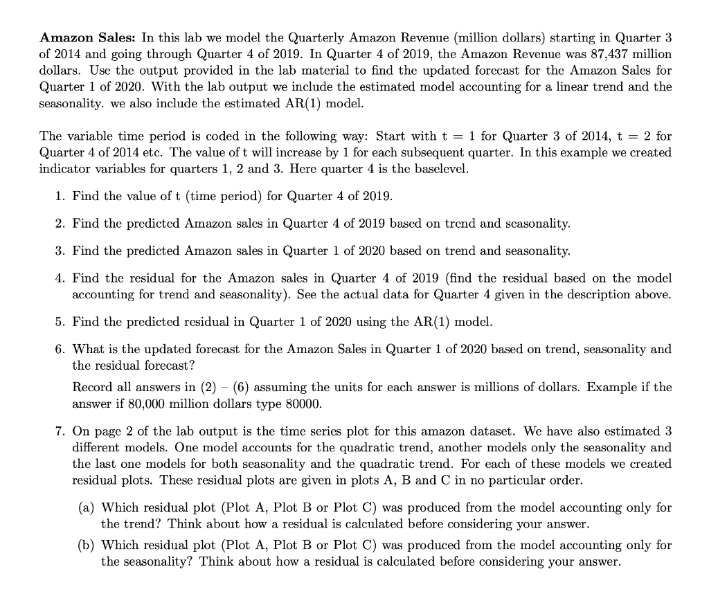
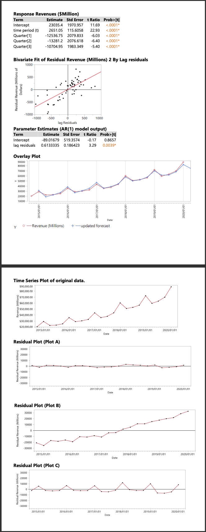
Amazon Sales: In this lab we model the Quarterly Amazon Revenue (million dollars) starting in Quarter 3 of 2014 and going through Quarter 4 of 2019. In Quarter 4 of 2019, the Amazon Revenue was 87,437 million dollars. Use the output provided in the lab material to find the updated forecast for the Amazon Sales for Quarter 1 of 2020. With the lab output we include the estimated model accounting for a linear trend and the seasonality. we also include the estimated AR(1) model. The variable time period is coded in the following way: Start with t = 1 for Quarter 3 of 2014, t = 2 for Quarter 4 of 2014 etc. The value of t will increase by 1 for each subsequent quarter. In this example we created indicator variables for quarters 1, 2 and 3. Here quarter 4 is the baselevel. 1. Find the value of t time period) for Quarter 4 of 2019. 2. Find the predicted Amazon sales in Quarter 4 of 2019 based on trend and seasonality. 3. Find the predicted Amazon sales in Quarter 1 of 2020 based on trend and seasonality. 4. Find the residual for the Amazon sales in Quarter 4 of 2019 (find the residual based on the model accounting for trend and seasonality). See the actual data for Quarter 4 given in the description above. 5. Find the predicted residual in Quarter 1 of 2020 using the AR(1) model. 6. What is the updated forecast for the Amazon Sales in Quarter 1 of 2020 based on trend, seasonality and the residual forecast? Record all answers in (2) - (6) assuming the units for each answer is millions of dollars. Example if the answer if 80,000 million dollars type 80000. 7. On page 2 of the lab output is the time series plot for this amazon dataset. We have also estimated 3 different models. One model accounts for the quadratic trend, another models only the seasonality and the last one models for both seasonality and the quadratic trend. For each of these models we created residual plots. These residual plots are given in plots A, B and C in no particular order. (a) Which residual plot (Plot A, Plot B or Plot C) was produced from the model accounting only for the trend? Think about how a residual is calculated before considering your answer. (b) Which residual plot (Plot A, Plot B or Plot C) was produced from the model accounting only for the seasonality? Think about how a residual is calculated before considering your answer. Response Revenues ($Million) Term Estimate Std Error t Ratio Prob>It| Intercept 23035.4 1970.957 11.69 <.0001 time period quarter bivariate fit of residual revenue by lag residuals dollars parameter estimates model output term estimate std errort ratio prob>It| Intercept -89.01679519.3574 -0.17 0.8657 lag residuals 0.6133335 0.186423 3.290.0039* Overlay Plot 90000 80000 70000 60000 > 50000 40000 30000 20000 10000 2015/01/01 2016/01/01 2017/01/01 2018/01/01 2019/01/01 2020/01/01 Y O Revenue (Millions) Date +-updated forecast Time Series Plot of original data. $90,000.00 $80,000.00 $70,000.00 $60,000.00 $50,000.00 $40,000.00 $30,000.00 $20,000.00 2015/01/01 2016/01/01 (Millions) 2017/01/01 2018/01/01 2019/01/01 2020/01/01 Date Residual Plot (Plot A) 30000 20000 $10000 50 Residual Revenue (Millions) 10000 S-20000 -30000 2015/01/01 2016/01/01 2017/01/01 2018/01/01 2019/01/01 2020/01/01 Date Residual Plot (Plot B) 30000 20000 10000 Residual Revenue (Millions) - 10000 -20000 - 30000 2015/01/01 2016/01/01 2017/01/01 2018/01/01 2019/01/01 2020/01/01 Date Residual Plot (Plot C) 30000 20000 10000 Residual Revenue Millions) -10000 -20000 -30000 2015/01/01 2016/01/01 2017/01/01 2018/01/01 2019/01/01 2020/01/01 Date Amazon Sales: In this lab we model the Quarterly Amazon Revenue (million dollars) starting in Quarter 3 of 2014 and going through Quarter 4 of 2019. In Quarter 4 of 2019, the Amazon Revenue was 87,437 million dollars. Use the output provided in the lab material to find the updated forecast for the Amazon Sales for Quarter 1 of 2020. With the lab output we include the estimated model accounting for a linear trend and the seasonality. we also include the estimated AR(1) model. The variable time period is coded in the following way: Start with t = 1 for Quarter 3 of 2014, t = 2 for Quarter 4 of 2014 etc. The value of t will increase by 1 for each subsequent quarter. In this example we created indicator variables for quarters 1, 2 and 3. Here quarter 4 is the baselevel. 1. Find the value of t time period) for Quarter 4 of 2019. 2. Find the predicted Amazon sales in Quarter 4 of 2019 based on trend and seasonality. 3. Find the predicted Amazon sales in Quarter 1 of 2020 based on trend and seasonality. 4. Find the residual for the Amazon sales in Quarter 4 of 2019 (find the residual based on the model accounting for trend and seasonality). See the actual data for Quarter 4 given in the description above. 5. Find the predicted residual in Quarter 1 of 2020 using the AR(1) model. 6. What is the updated forecast for the Amazon Sales in Quarter 1 of 2020 based on trend, seasonality and the residual forecast? Record all answers in (2) - (6) assuming the units for each answer is millions of dollars. Example if the answer if 80,000 million dollars type 80000. 7. On page 2 of the lab output is the time series plot for this amazon dataset. We have also estimated 3 different models. One model accounts for the quadratic trend, another models only the seasonality and the last one models for both seasonality and the quadratic trend. For each of these models we created residual plots. These residual plots are given in plots A, B and C in no particular order. (a) Which residual plot (Plot A, Plot B or Plot C) was produced from the model accounting only for the trend? Think about how a residual is calculated before considering your answer. (b) Which residual plot (Plot A, Plot B or Plot C) was produced from the model accounting only for the seasonality? Think about how a residual is calculated before considering your answer. Response Revenues ($Million) Term Estimate Std Error t Ratio Prob>It| Intercept 23035.4 1970.957 11.69 <.0001 time period quarter bivariate fit of residual revenue by lag residuals dollars parameter estimates model output term estimate std errort ratio prob>It| Intercept -89.01679519.3574 -0.17 0.8657 lag residuals 0.6133335 0.186423 3.290.0039* Overlay Plot 90000 80000 70000 60000 > 50000 40000 30000 20000 10000 2015/01/01 2016/01/01 2017/01/01 2018/01/01 2019/01/01 2020/01/01 Y O Revenue (Millions) Date +-updated forecast Time Series Plot of original data. $90,000.00 $80,000.00 $70,000.00 $60,000.00 $50,000.00 $40,000.00 $30,000.00 $20,000.00 2015/01/01 2016/01/01 (Millions) 2017/01/01 2018/01/01 2019/01/01 2020/01/01 Date Residual Plot (Plot A) 30000 20000 $10000 50 Residual Revenue (Millions) 10000 S-20000 -30000 2015/01/01 2016/01/01 2017/01/01 2018/01/01 2019/01/01 2020/01/01 Date Residual Plot (Plot B) 30000 20000 10000 Residual Revenue (Millions) - 10000 -20000 - 30000 2015/01/01 2016/01/01 2017/01/01 2018/01/01 2019/01/01 2020/01/01 Date Residual Plot (Plot C) 30000 20000 10000 Residual Revenue Millions) -10000 -20000 -30000 2015/01/01 2016/01/01 2017/01/01 2018/01/01 2019/01/01 2020/01/01 Date