An Exercise Science major implemented a 6-month exercise-training intervention where six athletes had their fitness level measured on three occasions: (1) prior to the intervention, (2) after 3 months, and (3) after 6 months. Their data are shown below. Higher scores indicate greater fitness level.ATHLETEPRE3 MONTH6 MONTH145505524242453364143439354055155596444956I entered the data above into SPSS and then I Conducted a Repeated-Measures ANOVA with PRE, 3-MONTHS and 6-MONTHS as the variables. I produced descriptive statistics, a graph and Post Hoc Contrasts. I Attached my SPSS output.I need to know 1. Is this statistically significant? Why or why not?2. If there are statistically significant differences, based on a Post Hoc Contrast, which TIME PERIODS are significantly different from which other TIME PERIODS, and how are they different?3. And finally I need to get someone's opinion or interpretation of WHY this outcome happened?

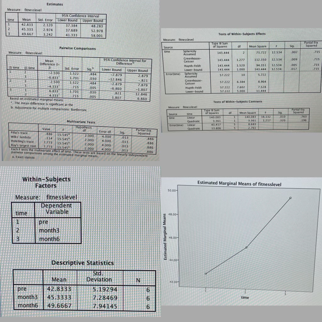
Estimates Measure: fitnesslevel 95%% Confidence Interval time Mean Std. Error Lower Bound | Upper Bound 1 42.833 2.120 37.384 48.283 45.333 2.974 37.689 52.978 49.667 3.242 41.333 58.001 Tests of within - Subjects Effects Measure: fitnesslevel Type Ill Sum Partial Et Source of Squares af Mean Square Sig Pairwise Comparisons time Sphericity 143.444 1.722 12.53 1002 1715 Measure: fitnesslevel Assumed Greenhouse 1009 .715 Mean onfidence Interval for Geisser 143.444 1.277 12.350 12.534 Difference (1- Difference Huynh-Feldt 143.444 1 520 4.351 12.534 715 ( time () time d. Error 12.534 017 Sig. Lower Bound Upper Bound Lower-boun 143.444 1.000 143.444 -2.500 1.522 -484 7.879 Sphericity Assumed 57.222 10 5.722 6.833 1.701 2.879 Error(time) .030 -12.846 2.500 .821 Greenhouse- 1.522 1484 Geisser 57.222 6.384 8.964 -2.879 4.333 .715 7.879 1005 7.602 1.701 -1.807 Huynh-Feldt 57.222 7.528 -6.860 6.833 57.222 5.000 11.44 .030 821 Lower-bound 4.333 1715 005 12.846 1.807 Based on estimated marginal means 6.860 Tests of Within-Subjects Contrasts *. The mean difference is significant at the Measure: fitnesslevel b. Adjustment for multiple comparisons: Bonferroni. Partial Eta Mean Square F Sig- Squared Source time time Linear 140.083 140.083 16.132 .010 -763 Quadratic 3.361 1.217 .320 196 Multivariate Tests 3.361 Error(time) Linear 43.417 8.683 Value Hypothesis Quadratic 13.806 2.761 Error df Partial Eta Pillar's trace -886 15.545* Sig. Squared Wilks' lambda .000 -114 4.000 15.545* .013 .886 Hotelling's trace 2.000 7.773 15.545 4.000 013 2.000 .886 Roy's largest root 7.773 15.545" 4.000 .013 2.000 .886 4.000 .013 Each F tests the multivariate effect of time. These tests are based on the linearly independent .886 pairwise comparisons among the estimated marginal means. a. Exact statistic Within-Subjects Estimated Marginal Means of fitnesslevel Factors 50.00 Measure: fitnesslevel Dependent time Variable 48.00- pre month3 Estimated Marginal Means month6 46.00- 44.00- Descriptive Statistics Mean Deviation 42.00 pre 42.8333 5.19294 month3 45.3333 7.28469 time month6 49.6667 7.94145