ANSWER MUST BE IN MATLAB CODE.

THANK YOU IN ADVANCE AND WILL RATE WELL....

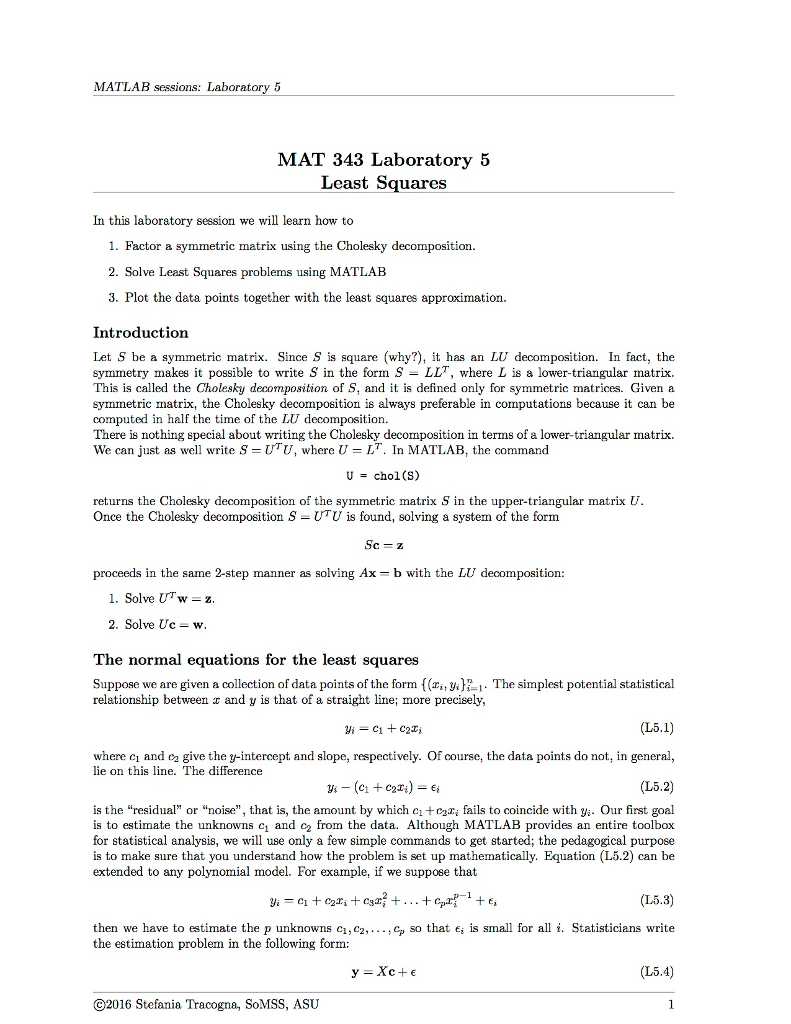
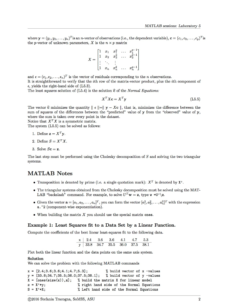
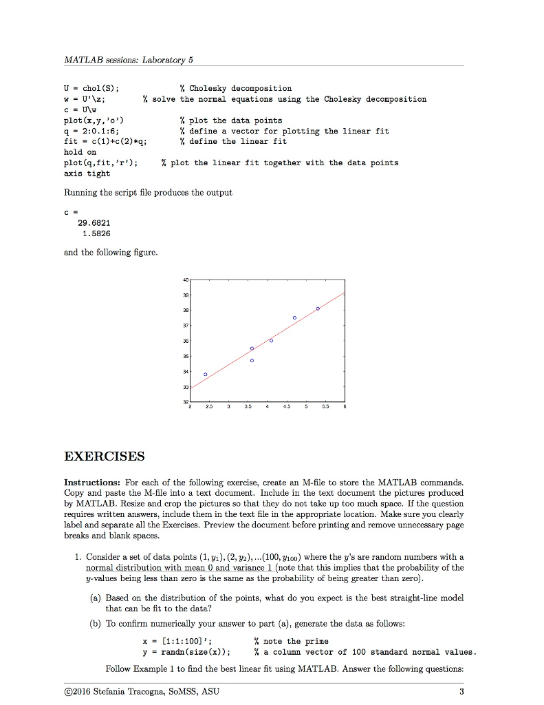
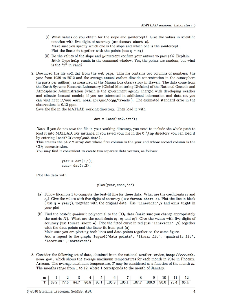
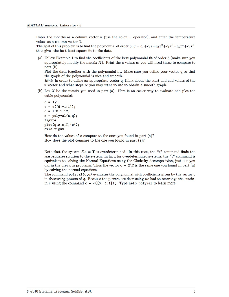
MATLAB sessions: Laboratory 5 MAT 343 Laboratory 5 Least Squares In this laboratory session we will learn how to 1. Factor a symmetric matrix using the Cholesky decomposition. 2. Solve Least squares problems using MATLAB 3. Plot the data points together with the least squares approximation. Introduction (why? Let S be a symmetric matrix. Since S is square t has an LU decomposition. In fact, the symmetry makes it possible to write S in the form S LLT, where L is a lower-triangular matrix. This is called the Cholesky decomposition of S, and it is defined only for symmetric matrices. Given a symmetric matrix, the Cholesky decomposition is always preferable in computations because it can be computed in half the time of the LU decomposition There is nothing special about writing the Cholesky decomposition in terms of a lower-triangular matrix. We can just as well write S UTU, where U L In MATLAB, the command U chol (S) returns the Cholesky decomposition of the symmetric matrix S in the upper-triangular matrix U Once the Cholesky decomposition S UTU is found, solving a system of the form Sc proceeds in the same 2-step manner as solving Ax b with the LU decomposition: 1. Solve UTw z 2. Solve Uc w. The normal equations for the least squares Suppose we are given a collection of data points of the form (r,, y 1. The simplest potential statistical relationship between z and y is that of a straight line; more precisely, (L5.1 where ci and c2 give the y-intercept and slope, respectively. Of course, the data points do not, in general e on this line. The difference 1 c2ri) (L5.2) s the residual" or "noise that is, the amount by which c c22:a fails to coincide with yi Our first is to estimate the unknowns c1 and ce from the data. Although MATLAB provides an entire toolbox for statistical analysis, we will use only a few simple commands to get started; the pedagogical purpose is to make sure that you understand how the problem is set up mathematically. Equation (L5.2) can be extended to any polynomial model. For example, if we suppose that L5.3 then we have to estimate the p unknowns ci,c2, ca so that Ei is small for all i. Statisticians write the estimation problem in the following form (L5.4 2016 Stefania Tracogna, SoMSS, ASU MATLAB sessions: Laboratory 5 MAT 343 Laboratory 5 Least Squares In this laboratory session we will learn how to 1. Factor a symmetric matrix using the Cholesky decomposition. 2. Solve Least squares problems using MATLAB 3. Plot the data points together with the least squares approximation. Introduction (why? Let S be a symmetric matrix. Since S is square t has an LU decomposition. In fact, the symmetry makes it possible to write S in the form S LLT, where L is a lower-triangular matrix. This is called the Cholesky decomposition of S, and it is defined only for symmetric matrices. Given a symmetric matrix, the Cholesky decomposition is always preferable in computations because it can be computed in half the time of the LU decomposition There is nothing special about writing the Cholesky decomposition in terms of a lower-triangular matrix. We can just as well write S UTU, where U L In MATLAB, the command U chol (S) returns the Cholesky decomposition of the symmetric matrix S in the upper-triangular matrix U Once the Cholesky decomposition S UTU is found, solving a system of the form Sc proceeds in the same 2-step manner as solving Ax b with the LU decomposition: 1. Solve UTw z 2. Solve Uc w. The normal equations for the least squares Suppose we are given a collection of data points of the form (r,, y 1. The simplest potential statistical relationship between z and y is that of a straight line; more precisely, (L5.1 where ci and c2 give the y-intercept and slope, respectively. Of course, the data points do not, in general e on this line. The difference 1 c2ri) (L5.2) s the residual" or "noise that is, the amount by which c c22:a fails to coincide with yi Our first is to estimate the unknowns c1 and ce from the data. Although MATLAB provides an entire toolbox for statistical analysis, we will use only a few simple commands to get started; the pedagogical purpose is to make sure that you understand how the problem is set up mathematically. Equation (L5.2) can be extended to any polynomial model. For example, if we suppose that L5.3 then we have to estimate the p unknowns ci,c2, ca so that Ei is small for all i. Statisticians write the estimation problem in the following form (L5.4 2016 Stefania Tracogna, SoMSS, ASU